

The MSRJD Response Functional
The Martin–Siggia–Rose–Janssen–de Dominicis construction turns a stochastic equation into a functional integral by enforcing the equation with a response field and retaining the functional determinant of the noise-to-field map. The determinant is constant only in special additive-noise, causal-discretization conventions.
Required background. Use Fokker–Planck evolution and Grassmann and Berezin integration.
Helpful background. Retarded, advanced, and Keldysh bases clarifies the parallel between response and statistical fields.
From the Langevin constraint to an action
Section titled “From the Langevin constraint to an action”Write additive Model A as
Insert the constraint and determinant as in Janssen 1976, pp. 378–379:
into the Gaussian noise average. Exponentiating the delta functional with a response field and integrating over gives, in a common convention,
The contour is chosen so the original Gaussian representation converges; equivalently one may rotate to a real response field and carry explicit factors of . The functional weight and source convention must be stated with the contour. Copying the action while changing reverses signs in response and noise terms.
The determinant can be represented by ghosts,
For additive noise with an Itô/prepoint discretization, the retarded Jacobian is triangular and often field independent, so ghosts decouple. With midpoint conventions, multiplicative noise, constraints, or nonlinear variable changes, the Jacobian contributes and cannot be discarded.
The response-action box is downstream of both the stochastic prescription and the probability evolution in the schematic. This ordering keeps the Jacobian, response-field contour, and equal-time prescription tied to the Langevin process they represent.
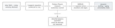
The MSRJD functional is an exact representation of the declared stochastic process only when response-field factors, Jacobian, boundary terms, and discretization convention are matched. It generates causal response and correlation functions but does not by itself impose equilibrium. Detailed balance may appear as an additional symmetry, and dynamic scaling requires a separate renormalization and slow-variable analysis. The diagram is schematic and not to scale.
The sections From the Langevin constraint to an action, Response and correlation functions, and Boundary terms and equal-time prescription give the text and equation equivalent of the response-action box.
Response and correlation functions
Section titled “Response and correlation functions”Couple a physical field through . Then
under the normalization above. Causality of the response-field propagator makes this vanish for . The correlator is statistical; vanishes in the elementary Gaussian theory, paralleling the Schwinger–Keldysh causal zero.
For the Gaussian mode , inversion gives
and noise contraction gives
With these reproduce the Langevin response and covariance.
Boundary terms and equal-time prescription
Section titled “Boundary terms and equal-time prescription”The initial probability distribution supplies a boundary action at . Integrations by parts in time can move terms to that boundary and change apparent time-reversal transformations. The retarded value is fixed by the stochastic discretization; setting it inconsistently changes tadpoles and the Jacobian.
For multiplicative noise , the determinant and noise kernel both depend on . The stochastic convention generates a drift correction. An MSRJD action missing that correction describes a different process even if its classical Langevin equation looks identical.
Use the stochastic and kinetic closure validity table to record the response contour, Jacobian, regulator, and stationarity checks.
Failure tests
Section titled “Failure tests”- Derive the determinant on the same discrete time lattice as the stochastic equation.
- Verify causal response against a finite source perturbation.
- Retain the initial boundary action.
- Change response-field contour only with all factors of transformed.
- For multiplicative noise, translate between Itô and Stratonovich and recover the same physical process.
- Check ghost decoupling rather than assuming it.
Exercise
Section titled “Exercise”Why is the Itô Jacobian field independent for with drift evaluated at ?
Solution
The discrete equation at step depends on the new variable only through . The Jacobian with rows ordered in time is triangular with constant diagonal , so its determinant is a field-independent normalization. Midpoint drift also depends on and changes the diagonal.
Continue
Section titled “Continue”Use the functional’s equilibrium time-reversal symmetry on detailed balance and fluctuation–dissipation and extend it carefully on generalized noise.
References
Section titled “References”- de Dominicis, C. (1976). “Techniques de renormalisation de la théorie des champs et dynamique des phénomènes critiques.” Journal de Physique Colloques 37(C1), C1-247–C1-253. DOI.
- Janssen, H.-K. (1976). “On a Lagrangean for Classical Field Dynamics and Renormalization Group Calculations of Dynamical Critical Properties.” Zeitschrift für Physik B 23, 377–380. DOI.
- Martin, P. C., Siggia, E. D., and Rose, H. A. (1973). “Statistical Dynamics of Classical Systems.” Physical Review A 8, 423–437. DOI.