

Hydrodynamization and the Kinetic-to-Hydrodynamic Map
Hydrodynamization is the emergence of a predictive constitutive description for the stress tensor and currents; it need not coincide with pressure isotropy, kinetic equilibrium, or a thermal density operator. A kinetic-to-hydrodynamic map is controlled when it conserves fluxes, preserves dissipative stresses and currents, quantifies residual nonhydrodynamic modes, and gives stable downstream observables over a switching window.
Required background. Validity of kinetic descriptions supplies the upstream domain, hydrodynamic attractors supplies the reduced late-time behavior, and initial conditions supplies the switching data. Helpful background. Gauge-theory EKT provides a controlled weak-coupling realization.
Four distinct milestones
Section titled “Four distinct milestones”For a local stress tensor with longitudinal and transverse pressures :
- Hydrodynamization means a truncated constitutive relation predicts to a stated accuracy.
- Isotropization means is small compared with a declared pressure scale.
- Kinetic equilibration means the one-particle distribution is close to a local equilibrium form, up to hydrodynamic perturbations.
- Thermalization is the stronger statement that relevant observables are described by a thermal state with the appropriate conserved charges.
In rapidly expanding systems, viscous hydrodynamics can work while remains far from one. Conversely, an accidentally isotropic stress tensor does not guarantee that higher moments have equilibrated.
Landau matching and dissipative data
Section titled “Landau matching and dissipative data”Given upstream , solve
for the Landau-frame velocity and energy density. With an EOS , define
Currents decompose as . The angle brackets denote the symmetric, transverse, traceless projection. Passing only and setting to zero erases physical nonequilibrium stress and creates a switching discontinuity.
On a general hypersurface, the minimum conservation condition is equality of normal fluxes:
Pointwise equality of the full tensors is preferable when both descriptions represent the same coarse-grained fields.
Nonhydrodynamic modes and a switching criterion
Section titled “Nonhydrodynamic modes and a switching criterion”Linearized kinetic theory separates slow conserved modes from a tower or continuum of faster modes. After transients decay, response to a perturbation can be approximated by hydrodynamic Green functions:
The residual defines an error, not a field to silently discard. Practical diagnostics include
Small values are helpful but not individually sufficient; the constitutive residual and observable stability matter. Hydrodynamic attractors explain why a resummed constitutive description can work before a conventional gradient series converges Heller and Spaliński 2015.
A robust switch is a window: vary , matching prescription, and upstream/downstream truncation while keeping the physical setup fixed. If downstream observables move more than the claimed uncertainty, switching dependence is part of the error budget.
A controlled weak-coupling example
Section titled “A controlled weak-coupling example”In a boost-invariant conformal kinetic system, the relaxation variable compares expansion to microscopic relaxation. EKT calculations show convergence of suitably scaled stress evolution toward a universal response before full pressure isotropy, and KoMPoST transports perturbations to hydrodynamics Kurkela et al. 2019. This demonstrates a kinetic-to-hydrodynamic map in that weak-coupling model. It does not establish that the same numerical switch time applies to QCD at all collision energies.
Failure cases
Section titled “Failure cases”Hydrodynamics is unreliable if no physical timelike Landau eigenvector exists, dissipative corrections make the truncation uncontrolled, conserved fluxes jump, the EOS has no matching composition, or residual nonhydrodynamic response remains large. Negative longitudinal pressure by itself is not a universal veto, but it demands a formulation whose constitutive approximation remains demonstrably predictive.
Hydrodynamization is the matching edge between the pre-equilibrium and viscous-hydrodynamic nodes, not a claim of local equilibrium.
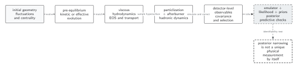
At the central matching edge, a timelike Landau eigenvector defines the local energy density and flow, while shear stress, bulk pressure, and conserved currents carry the nonideal remainder. Conservation across the switching surface and stability under switching-time variation are essential. The downstream nodes explain why acceptable matching is judged by predictive observables, not by isotropic pressure alone. The diagram is schematic and not to scale.
The corresponding text procedure is to reconstruct all matched hydrodynamic fields, test inverse Reynolds and gradient measures together with residual nonhydrodynamic response, preserve conserved fluxes, and repeat the calculation over a defensible switching window.
Exercises
Section titled “Exercises”1. Bjorken pressures. For in the local rest frame and equilibrium pressure , express the bulk pressure and one independent shear component.
Solution
The average pressure is , so . A convenient shear scalar is , giving and .
2. Switching test. Two switch times give identical total energy but different final . Is conservation sufficient?
Solution
No. Conservation is necessary, but different treatment of shear stress, transverse flow, or residual modes can change anisotropic response. The variation is a matching systematic until convergence or a correction model accounts for it.
Continue to viscous hydrodynamics, particlization, and afterburners.
References
Section titled “References”- Heller, Michał P., and Michał Spaliński. “Hydrodynamics Beyond the Gradient Expansion: Resurgence and Resummation.” Physical Review Letters 115, no. 7 (2015): 072501. DOI.
- Kurkela, Aleksi, Aleksas Mazeliauskas, Jean-François Paquet, Sören Schlichting, and Derek Teaney. “Matching the Nonequilibrium Initial Stage of Heavy Ion Collisions to Hydrodynamics with QCD Kinetic Theory.” Physical Review Letters 122, no. 12 (2019): 122302. DOI.
- Romatschke, Paul. “Relativistic Fluid Dynamics Far from Local Equilibrium.” Physical Review Letters 120, no. 1 (2018): 012301. DOI.