Spectral Functions and Transport Peaks

A transport spectrum may contain an exact delta function from a conserved overlap, a finite-width relaxation peak, a hydrodynamic pole whose width scales with momentum, a quasiparticle resonance, or a branch cut from a continuum or long-time tail. These objects have different analytic origins and different limiting behavior. A narrow feature is not evidence for a quasiparticle until its volume, resolution, and conservation-law dependence have been tested.

Required background. Sources, linear response, and Kubo formulae fixes $G_R$, $\rho=-2\operatorname{Im}G_R$, and the physical response. Spectral positivity and sum rules supplies the Lehmann representation. Helpful background. Long-time tails and fluctuation renormalization derives nonanalytic low-frequency terms that no finite pole sum reproduces.

Analytic structures and what they mean

For a Hermitian bosonic operator, a retarded pole at

$$\omega_\star(\mathbf k)=\Omega(\mathbf k)-i\Gamma(\mathbf k), \qquad \Gamma>0,$$

lies below the real axis. If $\Gamma\ll\Omega$ and the pole is isolated from other singularities, it can describe a long-lived quasiparticle. A purely imaginary pole can instead be a relaxation or diffusion mode; it need not correspond to a propagating particle.

A branch cut represents a continuum of spectral weight or the accumulation of singularities in an infinite system. Threshold continua have nonanalytic endpoints. Hydrodynamic fluctuations generate cuts reaching the origin. An exact real-axis delta function is more singular still: it usually records a conserved overlap or a stable excitation, not a peak with an unmeasured small width.

At finite volume, the exact spectrum is a sum of discrete lines. Poles and cuts of thermodynamic-limit response emerge only after the volume limit and a specified analytic or coarse-graining prescription. Artificially convolving those lines with a kernel of width $\epsilon$ produces a resolution-broadened spectrum; stability as $\epsilon$ and volume are varied is required before assigning a physical width.

The pole, cut, and hydrodynamic-mode classification is developed in Forster 1995, chs. 3–6 and Hartnoll, Lucas, and Sachdev 2018, ch. 2, Open PDF; lattice transport examples illustrating finite resolution are reviewed in Meyer 2011, §§3–4, Open PDF.

Drude weight versus a relaxation peak

A single nearly conserved current component gives the model

$$\sigma(\omega)=\frac{D_{\mathrm D}}{\Gamma-i\omega} +\sigma_{\mathrm{inc}}(\omega),$$

so

$$\operatorname{Re}\sigma(\omega) =D_{\mathrm D}\frac{\Gamma}{\Gamma^2+\omega^2} +\operatorname{Re}\sigma_{\mathrm{inc}}(\omega).$$

For fixed $D_{\mathrm D}$, the peak has height $D_{\mathrm D}/\Gamma$, width $\Gamma$, and area $\pi D_{\mathrm D}$ on the whole real axis. As $\Gamma\to0^+$,

$$\operatorname{Re}\sigma(\omega) \longrightarrow \pi D_{\mathrm D}\delta(\omega) +\operatorname{Re}\sigma_{\mathrm{inc}}(\omega).$$

The limit preserves spectral weight while the dc value diverges. $D_{\mathrm D}$, $\Gamma$, and $\sigma_{\mathrm{inc}}$ are separately meaningful only if the data resolve the peak and if the chosen slow-mode decomposition is justified. Two overlapping relaxation scales can produce a visibly non-Lorentzian feature.

A hydrodynamic pole and its residue

For diffusion, the density retarded function in the site’s convention is

$$G_R^{nn}(\omega,\mathbf k) =-\chi\frac{Dk^2}{-i\omega+Dk^2},$$

and therefore

$$\rho_{nn}(\omega,\mathbf k) =\frac{2\chi Dk^2\omega}{\omega^2+(Dk^2)^2}.$$

The pole width $Dk^2$ vanishes because density is conserved, while the numerator also vanishes as $k^2$. This residue is essential: setting $k=0$ too early removes the finite-frequency density response. The equal-time fluctuation is recovered by the thermal sum rule, while the two noncommuting limits reproduce static susceptibility and charge conservation.

Sound gives paired poles $\omega=\pm c_sk-i\Gamma_sk^2/2+\cdots$. A quasiparticle peak can have a similar shape at a fixed momentum, but hydrodynamic identification requires the predicted small-$k$ dispersion, residue, and channel relations—not merely a Lorentzian fit.

Cuts and non-Lorentzian low-frequency weight

If an equilibrium correlation decays as $t^{-d_s/2}$, Fourier transformation gives a nonanalytic contribution. In three spatial dimensions a stress retarded function contains a term proportional to $(-i\omega)^{3/2}$, and the effective viscosity acquires an $(-i\omega)^{1/2}$ correction. This is a branch point at the origin, so no finite set of relaxation poles reproduces the asymptotic analytic structure Kovtun and Yaffe 2003, §§III–IV, Open PDF.

Thresholds and multiparticle continua can likewise overlap a transport feature. A fit that assigns all low-frequency weight to one Lorentzian can then bias both the width and the dc slope while still describing Euclidean data well.

Resolution-aware classification

Use three tests before naming a feature:

1. Analytic test: does a controlled equation locate a pole, a cut, or an exact conserved projection?
2. Scaling test: how do position, width, residue, and area change with momentum, symmetry breaking, volume, and regulator?
3. Resolution test: can the forward kernel distinguish that structure from alternatives satisfying the same contacts, positivity, and sum rules?

The transport-extraction covariance reference states the required resolution, covariance, window, and volume record. Transport sum rules provide integral checks but cannot by themselves decide how weight is distributed within an unresolved window.

The middle and lower branch of the diagram summarize the classification problem. Inspect the spectral-constraint box together with the unresolved-peak warning: a pole, a delta function, a cut, and a narrow but finite peak can satisfy similar integral constraints while supporting different transport claims.

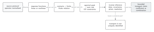
Analytic structure and scaling determine whether low-frequency weight is a hydrodynamic pole, an exact Drude delta function, a relaxation peak, or a continuum. Sum rules and ultraviolet information constrain total weight but do not resolve its distribution. The diagram is schematic; the non-identification branch is a valid conclusion, not a failed fit.

In text: locate singularities in the retarded function, track residue and width with momentum, breaking, volume, and regulator, and pass the candidate structures through the actual forward kernel and covariance. Name only the spectral feature that those three tests distinguish.

Exercise: conserved weight in the Drude limit

Show that the Lorentzian part of $\operatorname{Re}\sigma$ has an area independent of $\Gamma$, and derive its distributional limit.

Solution

Direct integration gives

$$\int_{-\infty}^{\infty}d\omega\, D_{\mathrm D}\frac{\Gamma}{\Gamma^2+\omega^2} =\pi D_{\mathrm D}.$$

For any smooth test function $f$,

$$\lim_{\Gamma\to0^+}\int d\omega\, f(\omega)\frac{\Gamma}{\Gamma^2+\omega^2} =\pi f(0),$$

which is precisely $\Gamma/(\Gamma^2+\omega^2)\to\pi\delta(\omega)$. The width tends to zero and the height diverges, but the area remains fixed. A numerical broadening kernel can imitate this shape without determining whether $\Gamma$ is physical.

References

• Forster, Dieter. 1995. Hydrodynamic Fluctuations, Broken Symmetry, and Correlation Functions. Advanced Book Classics. Boca Raton, FL: CRC Press. DOI.
• Hartnoll, Sean A., Andrew Lucas, and Subir Sachdev. 2018. Holographic Quantum Matter. Cambridge, MA: MIT Press. Open PDF.
• Kovtun, Pavel, and Laurence G. Yaffe. 2003. “Hydrodynamic Fluctuations, Long-Time Tails, and Supersymmetry.” Physical Review D 68 (2): 025007. DOI. Open PDF.
• Meyer, Harvey B. 2011. “Transport Properties of the Quark–Gluon Plasma: A Lattice QCD Perspective.” European Physical Journal A 47: 86. DOI. Open PDF.

Diffusion, Conductivity, and Susceptibility turns the diffusive pole into a matrix Einstein relation. Transport Extraction, Inverse Problems, and Error Budgets tests whether a dataset actually resolves any proposed peak.