Spectral and Statistical Evolution

The spectral function describes which excitations and commutator response are available; the statistical function describes how the state populates and coherently combines them. Their coupled evolution is demonstrated explicitly in Aarts and Berges 2001, §§ II–III. A time-dependent occupation number is a derived diagnostic only when a quasiparticle or other reconstruction ansatz has been tested.

Required background. Use the Kadanoff–Baym equations for their coupled dynamics and causal and statistical propagators for canonical normalization.

Helpful background. Spectral and real-time functional methods discuss analytic continuation and positivity assumptions beyond the present initial-value setting.

Distinct data and exact constraints

For a real scalar field,

$$F(x,y)=\frac12\langle\{\phi(x),\phi(y)\}\rangle, \qquad \rho(x,y)=i\langle[\phi(x),\phi(y)]\rangle.$$

$F$ is symmetric and state dependent; $\rho$ is antisymmetric and fixed at equal time by the canonical algebra, though its later shape is interaction and state dependent. The indispensable sum rules are local in time:

$$\rho_{\mathbf p}(t,t)=0, \qquad \partial_t\rho_{\mathbf p}(t,t')|_{t=t'}=1.$$

For a sufficiently long relative-time transform, define the real spectral density $\mathcal A(X,p)=-i\rho_W(X,p)$. The corresponding first moment is

$$\int\frac{dp^0}{2\pi}\,p^0\mathcal A(X,p)=1,$$

subject to the Fourier and window conventions. Near a finite initial boundary, the equal-time condition is more reliable because a truncated transform distorts the moment.

Widths and occupations

Near a well-isolated weakly damped mode, a useful ansatz is

$$\mathcal A(X,p)\simeq \frac{2p^0\Gamma(X,\mathbf p)} {[(p^0)^2-\Omega^2(X,\mathbf p)]^2+[p^0\Gamma(X,\mathbf p)]^2},$$

with conventions stated for $\Gamma$. If $F_W$ has the same resolved shape, one may define

$$F_W(X,p)=-i\left(\frac12+f(X,p)\right)\rho_W(X,p)$$

for bosons. Away from KMS equilibrium, $f$ can depend on the sign of $p^0$, need not be positive under every projection, and need not reduce to a single on-shell number. Overlapping peaks, broad continua, coherent off-diagonal components, or short Wigner windows make the extraction ambiguous.

The width is not simply the decay rate of an equal-time observable. Spectral damping concerns relative-time response; relaxation of $F(t,t)$ occurs in center time and can be governed by different eigenmodes. A finite volume can dephase for many oscillation periods and later recur without any irreversible information loss.

The hierarchy keeps spectral and statistical evolution together in the same two-time box because neither can generally be reconstructed from the other away from equilibrium. A quasiparticle occupation is a later shell approximation, not the definition of $F$.

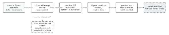
The spectral function carries commutator support, widths, and exact equal-time normalization, while the statistical function carries state-dependent fluctuations. A self-energy closure couples their evolution. Reduction to a distribution requires preservation of the spectral sum rule and a controlled width, gradient, and memory approximation; equilibrium KMS is a special relation, not a generic closure. The diagram is schematic and not to scale.

The sections Distinct data and exact constraints, Widths and occupations, and Coupled evolution and interpretation supply the text and equation equivalent of the two-time box and the conditions for leaving it.

Checked free and damped limits

For a free mode,

$$\rho(t,t')=\frac{\sin[\omega(t-t')]}{\omega}, \qquad F(t,t')=\frac{n+\tfrac12}{\omega}\cos[\omega(t-t')].$$

The spectral peaks are delta functions at $p^0=\pm\omega$, while the ratio of $F_W$ to $\rho_W$ returns $n+1/2$ after treating the two signs consistently. There is no width and no center-time evolution.

For a phenomenological damped response $\rho(s)=e^{-\Gamma|s|/2}\sin(\Omega s)/\Omega$, the equal-time derivative remains one, but the Fourier peaks broaden by order $\Gamma$. Cutting the transform at $|s|<s_{\max}$ adds an artificial resolution width of order $1/s_{\max}$. Therefore a claimed physical width must remain stable as $s_{\max}$ and the window profile are varied.

Coupled evolution and interpretation

$\Sigma_\rho$ modifies causal propagation and spectral width; $\Sigma_F$ carries fluctuations and gain terms. In a self-consistent closure each is a functional of both $F$ and $\rho$, so evolving $F$ on a frozen equilibrium spectrum omits spectral feedback. Such a kinetic approximation can be controlled, but only by comparing it with the coupled solution.

Thermalization requires more than a late-time exponential-looking $F$. Evidence includes time-translation invariance over an expanding window, the KMS relation between $F$ and $\rho$, agreement of temperatures extracted from independent observables, conservation of the closed-system charges, and stability against volume and truncation changes. A finite 2PI truncation may approach a stationary state whose detailed properties differ from the exact theory.

Failure tests

1. Monitor the equal-time spectral conditions mode by mode, not just their momentum average.
2. Vary Wigner center time, relative-time window, and window shape independently.
3. Compare at least two occupation reconstructions—for example equal-time covariance and spectral-ratio fits—and state where they disagree.
4. Increase volume until recurrences lie beyond the claimed relaxation interval.
5. Apply the conservation and numerical validation matrix before fitting an equilibrium distribution.

Exercise

For the free mode, show that the equal-time estimator

$$n_{\mathrm{eff}}+\frac12= \sqrt{F(t,t)\,\partial_t\partial_{t'}F(t,t')|_{t=t'}}$$

returns $n+1/2$. Give one reason it may fail in an interacting system.

Solution

$F(t,t)=(n+1/2)/\omega$ and the mixed derivative is $\omega(n+1/2)$, so their product is $(n+1/2)^2$. In an interacting system a broad or multi-peak spectrum has no unique frequency relating field and momentum variances; squeezing or anomalous coherence also invalidates the one-number reconstruction.

Continue

Use numerical validation to distinguish genuine spectral broadening, truncation effects, finite-window resolution, and discretization drift.

References

• Aarts, G., and Berges, J. (2001). “Nonequilibrium Time Evolution of the Spectral Function in Quantum Field Theory.” Physical Review D 64, 105010. arXiv:hep-ph/0103049; DOI.
• Berges, J., and Cox, J. (2001). “Thermalization of Quantum Fields from Time-Reversal Invariant Evolution Equations.” Physics Letters B 517, 369–374. arXiv:hep-ph/0006160; DOI.