

Renormalization of Open Effective Dynamics
Renormalizing an open effective field theory requires a doubled operator basis: ultraviolet modes can renormalize coherent propagation, damping, noise, and higher jump structures together. Trace normalization restricts the basis to terms that vanish when the two contour histories coincide, while complete positivity imposes inequalities that are stronger than those linear identities. A consistent loop calculation must preserve the former and explicitly test the latter at every scale and truncation.
Required background. Trace, positivity, and causal consistency supplies the regulated identities to preserve. Counterterms, subdivergences, and locality supplies the vacuum renormalization logic. Helpful background. Driven criticality shows how coherent and dissipative couplings enter an infrared RG problem.
The doubled operator basis
Section titled “The doubled operator basis”Write a local open action as
In the basis, a derivative and field expansion for one real scalar begins schematically as
Every term contains at least one field, ensuring . Contour reality makes coefficients of terms even in purely imaginary in this convention and constrains those odd in . Noise positivity requires the quadratic form beginning with and to be nonnegative over the EFT momentum range. Nonlinear complete positivity imposes additional relations among the higher- vertices when they are to arise from a Kossakowski factorization.
One cannot renormalize only the retarded inverse propagator. Loops involving , , and mix response and fluctuation sectors, and an operator absent at matching can be generated if no symmetry forbids it. The working basis must include all local doubled operators at the target order in fields, derivatives, coupling, and -field counting.
A one-loop scalar calculation
Section titled “A one-loop scalar calculation”Consider the relaxational scalar model
Its action is a special open field theory with damping and Gaussian noise. The free equal-time correlator is
Contracting two legs of the vertex gives the one-loop tadpole
The factor counts the contracted choices. The divergence is local and is removed by a counterterm already in the basis. This calculation shows two open-system features: the loop uses the statistical correlator, and its divergence must be canceled without generating a forbidden all- term. In a general driven theory and are independent, additional diagrams renormalize them and the interaction vertices independently, and no thermal Einstein relation may be imposed unless protected by a dynamical symmetry.
A practical loop calculation proceeds as follows.
- Regulate momentum, frequency, and any initial-time boundary consistently on both contour branches.
- List all operators allowed at the desired order.
- Compute divergent 1PI vertices with their indices retained.
- Subtract subdivergences before testing locality of the remaining divergence.
- Fit counterterms inside the allowed doubled basis.
- Verify normalization, reality, causal zeros, symmetry Ward identities, and the positivity inequalities.
- Match renormalized couplings to reduced observables and vary the scheme and scale within the truncation error.
The explicit one-loop open construction of Avinash et al. 2017, §§3–5 found that its trace-preserving “Lindblad conditions” form an RG-invariant subspace in that model. This is a model- and order-specific result, not a theorem that arbitrary open scalar truncations remain completely positive.
Constraint surfaces and positivity cones
Section titled “Constraint surfaces and positivity cones”Let linear normalization and reality conditions be for couplings . An RG flow remains on that constraint surface only if
This tangency condition can be checked algebraically from the beta functions. It is the appropriate test for trace identities and symmetry relations.
Complete positivity usually defines a cone rather than a linear surface—for example or a positive Kossakowski matrix. Tangency to does not keep the flow inside that cone. At its boundary, require the beta function to point inward or tangent in the chosen coordinates, and account for operators omitted by the truncation. Scheme redefinitions can change individual coordinates; physical reduced correlators and the existence of a positive representation over a declared scale interval are the meaningful outputs.
Exact Wilsonian coarse-graining of a density operator can itself be organized as a quantum channel. A current preprint represents a particular exact RG flow by a Lindbladian in scale Goldman, Lashkari, and Leigh 2024. That scale generator is not physical-time dissipation, and its channel property does not prove that a separately truncated real-time open EFT has a CPTP continuum limit.
Nonlocal divergences and initial-state terms
Section titled “Nonlocal divergences and initial-state terms”Ordinary EFT renormalizability relies on ultraviolet divergences being expressible as local operators consistent with symmetry. Open reductions add possible initial-time boundary operators, state dependence, and nonlocal kernels. A sufficiently regular state often shares the local short-distance singularities used by vacuum counterterms, while a singular preparation or a sharp system–environment split can introduce additional boundary divergences.
If a loop produces a nonpolynomial divergent dependence on external momentum or frequency after subdivergences are removed, a finite local basis cannot absorb it. The options are to retain a nonlocal kernel with its own matching, enlarge the degrees of freedom, or conclude that the proposed local truncation is not closed. The open-Yukawa calculation of Avinash, Jana, and Rudra 2019 reported nonlocal one-loop fermion self-energy divergences despite imposing tree-level trace conditions. Because that result is a preprint and model-specific, it is best treated as a concrete warning and calculation to reproduce, not a universal obstruction.
Gauge theories require a regulator and counterterms compatible with the physical constraint identities. A gauge-variant dissipative counterterm cannot be justified merely because it cancels a gauge-fixed two-point divergence. Match on gauge-invariant observables or derive the appropriate BRST/constraint identities for the doubled theory.
EFT error and the continuum claim
Section titled “EFT error and the continuum claim”A renormalized open EFT prediction should state
with the derivative order , loop order , matching scale, memory approximation, and initial-state uncertainty identified. Residual and regulator dependence should be smaller than the retained EFT error after matching.
Showing that a finite set of couplings remains in a positivity cone over a finite scale interval is useful evidence. It does not establish a UV-complete Lindblad QFT: new operators can enter, the local Markov expansion can fail, and an infinite-dimensional semigroup may lack the required domain. The canonical open-dynamics consistency and evidence matrix keeps these conclusions distinct.
Common failure modes
Section titled “Common failure modes”Renormalizing response but not noise. Keldysh loops mix sectors; retain every allowed counterterm at the working order.
Using normalization as a positivity proof. Linear contour identities do not imply a positive Kossakowski matrix.
Calling every RG Lindbladian physical time evolution. Coarse-graining scale and laboratory time are different parameters with different interpretations.
Hiding a nonlocal divergence in a running local coupling. Test the full external momentum and frequency dependence after subdivergence subtraction.
Renormalization acts on the open action or generator after the reduced dynamics has been defined; it does not replace the microscopic and positivity checks shown at the ends of the diagram.
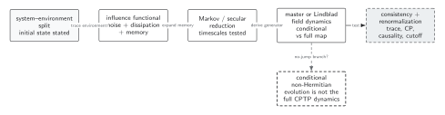
The solid sequence emphasizes that renormalization belongs to the consistency analysis of an already specified reduced theory. Local operators on the doubled contour can mix, while nonlocal divergences expose a failure of the assumed local basis. Complete positivity at one cutoff is not by itself a continuum theorem, and the dashed no-jump branch is not the full CPTP evolution. The diagram is schematic and does not identify RG scale with physical time.
The text equivalent is a two-part test: close the coherent, dissipative, and noise operator basis under renormalization, including its frequency dependence, and independently verify that the renormalized map preserves trace, Hermiticity, positivity, and causal response.
Exercises
Section titled “Exercises”Derive the tangency condition for an RG-invariant trace constraint.
Solution
Along the flow, . The chain rule gives . If this vanishes whenever , a trajectory starting on the constraint surface remains there to the calculated order. A nonzero result identifies a missing counterterm, a symmetry-breaking regulator, or a calculation error.
Why does and preservation of all trace identities not guarantee ?
Solution
Trace identities constrain linear combinations of doubled couplings but do not fix the sign of the noise coefficient. If points outward at , the truncated flow crosses into negative noise. One must test the positivity boundary, include generated operators, and determine whether the crossing is physical or a truncation or scheme artifact.
Continue to controlled applications
Section titled “Continue to controlled applications”A reproducible calculation tests running constraints and cutoff dependence in a bounded model. Critical long-distance applications return to driven steady states; microscopic derivations begin with influence functionals.
References
Section titled “References”- Avinash, Chandan Jana, R. Loganayagam, and Arnab Rudra. “Renormalization in Open Quantum Field Theory. Part I. Scalar Field Theory.” Journal of High Energy Physics 2017, no. 11 (2017): 204. doi:10.1007/JHEP11(2017)204. Open preprint.
- Avinash, Chandan Jana, and Arnab Rudra. “Renormalisation in Open Quantum Field Theory II: Yukawa Theory and Passarino–Veltman Reduction.” arXiv preprint (2019). arXiv:1906.10180.
- Goldman, Samuel, Nima Lashkari, and Robert G. Leigh. “A Lindbladian for Exact Renormalization of Density Operators in QFT.” arXiv preprint (2024). arXiv:2410.16582.
- Nagy, Sandor, and Janos Polonyi. “Renormalizing Open Quantum Field Theories.” Universe 8 (2022): 127. doi:10.3390/universe8020127.
- Wilson, Kenneth G., and John Kogut. “The Renormalization Group and the Expansion.” Physics Reports 12 (1974): 75–200. doi:10.1016/0370-1573(74)90023-4.