

Nonthermal Fixed Points and Wave Turbulence
Far from equilibrium, a field can transport approximately conserved quantities across momentum scales while its correlators evolve self-similarly. A nonthermal fixed point is supported when a common scaling function, conservation-law exponent relations, an extended inertial window, and attraction from more than one initial condition survive regulator and finite-size tests. A transient visual collapse by itself establishes only a useful rescaling.
Required background. Equilibration and dephasing distinguishes scaling evolution from near-stationarity. Spectral and statistical evolution defines the two-point functions whose scaling is tested. Helpful background. Transport equations supply weak-turbulence closures, and quenches, coarsening, and aging provide a related but distinct real-space scaling language.
Self-similar evolution and exponent constraints
Section titled “Self-similar evolution and exponent constraints”For an isotropic occupation or statistical correlator, choose a reference time and test
Here moves a characteristic scale toward the infrared as ; moves it toward the ultraviolet. The convention must be stated because some literature places the inverse power inside .
Suppose
is conserved within the scaling window. Changing variables to gives
Therefore conservation requires
Particle transport has . For quasiparticle energy , energy transport has . If one scaling form appears to conserve both quantities with , either two cascades occupy different momentum windows or the assumptions are inconsistent.
Flux distinguishes a cascade from a drifting spectrum
Section titled “Flux distinguishes a cascade from a drifting spectrum”A kinetic equation has the form
For a conserved density, integrate over a momentum ball to define
and a radial flux by
An inertial cascade exhibits a momentum interval in which forcing and sinks are negligible and is approximately independent of . Its sign fixes the direction. A fitted power law without a flux plateau can instead be a moving cutoff, crossover, or finite-time deformation.
Weak wave turbulence derives stationary spectra from the homogeneity of and assumes weak nonlinear broadening, random phases, and scale locality of the collision integral. Strongly occupied infrared fields can violate those assumptions; classical-statistical simulations, large- expansions, functional methods, or defect descriptions then provide different controlled windows. The real-time functional approach to nonthermal fixed points is developed by Berges and Hoffmeister 2009, while simulations and large- calculations demonstrate model-dependent realizations rather than a theorem of universal attraction.
A reproducible collapse test
Section titled “A reproducible collapse test”Given measurements , choose before fitting and form
Fit one common curve using the full covariance across momenta and times. Then test:
- whether the same predicts held-out times;
- whether agrees with zero for the independently measured conserved quantity;
- whether the inferred flux has a scale-independent interval;
- whether the interval grows rather than merely shifts with lattice cutoff or box size; and
- whether distinct initial conditions approach the same after nonuniversal time and amplitude rescalings.
This separates an inference problem from an eye-guided collapse. Covariance matters because neighboring momentum bins and common normalization errors can make many exponent pairs look acceptable.
Classicality, defects, and quantum control
Section titled “Classicality, defects, and quantum control”Large occupation can suppress quantum vertices relative to classical-statistical ones, but the approximation must fail as the cascade reaches modes with . Ultraviolet cascades therefore encounter a quantum or regulator boundary. Infrared inverse cascades can encounter condensate formation, finite volume, or topological defects. Defect densities may control a scaling function without a weak-wave kinetic description.
Large- evolution avoids a small-coupling assumption in some models and has shown nonthermal scaling beyond the simplest classical-statistical window Berges and Wallisch 2017. That result is evidence for a broader mechanism in a specified theory and expansion, not a model-independent exponent table. Platform-specific realizations and their current evidence belong in Volume XII.
Failure modes and supported conclusions
Section titled “Failure modes and supported conclusions”One decade is not automatically an inertial range. Vary the forcing, sink, initial scale, cutoff, and volume; the proposed universal window should separate from all of them.
Conservation inferred from fitted exponents. Measure the conserved integral and boundary flux independently. Otherwise the exponent relation is circular.
Transient collapse promoted to a fixed point. Demonstrate attraction from multiple initial conditions and widening scale separation.
Classical evolution promoted to quantum universality. Track occupancies and compare with a quantum-controlled expansion or correction where the classicality criterion fails.
Power-law tails without covariance. Correlated bins can make a slope appear much more precise than it is.
Use the upper row to distinguish a self-similar nonthermal fixed-point regime from a prethermal plateau or an ETH-controlled stationary state. The lower chaos observables are not prerequisites for establishing wave-turbulent scaling.
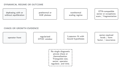
Nonthermal fixed-point evidence requires stable scaling exponents, collapse over expanding time and momentum windows, and the correct conserved flux. The diagram is schematic: its upper nodes are alternatives rather than an evolution sequence, and the independent lower row does not make scaling behavior a chaos diagnosis.
In text-equivalent form, establish scaling from the measured distribution and its conservation laws, then test cutoff, volume, initial-condition, and fitting-window dependence. ETH matrix elements and OTOC or spectral diagnostics address different claims.
Exercises
Section titled “Exercises”For a relativistic ultraviolet energy cascade with , derive the conservation relation.
Solution
Energy corresponds to , so conservation gives . An ultraviolet-moving scale has in this page’s convention, hence : occupancy at fixed rescaled shape decreases while energy moves to larger momentum.
A collapse passes for but fails at the earliest time and at momenta within two bins of both cutoffs. State a defensible fit protocol.
Solution
Predeclare a time interval after the transient and a momentum interval separated from the infrared and ultraviolet cutoffs, fit with the restricted covariance matrix, then vary both boundaries and repeat at larger and finer spacing. Report exponent drift as a systematic error; do not use the excluded regions to enlarge the claimed scaling window.
Continue to eigenstate and model tests
Section titled “Continue to eigenstate and model tests”ETH asks a different question about stationary matrix elements in generic finite systems. Thermalization and prethermalization treats charge-constrained plateaus. Testing a scaling collapse requires numerical data and negative controls matched to the model and time window.
References
Section titled “References”- Berges, Jürgen, and Gabriele Hoffmeister. “Nonthermal Fixed Points and the Functional Renormalization Group.” Nuclear Physics B 813 (2009): 383–407. doi:10.1016/j.nuclphysb.2008.12.017. Open preprint.
- Berges, Jürgen, Alexander Rothkopf, and Jonas Schmidt. “Nonthermal Fixed Points from the Functional Renormalization Group.” Physical Review Letters 101 (2008): 041603. doi:10.1103/PhysRevLett.101.041603. Open preprint.
- Berges, Jürgen, and Benjamin Wallisch. “Nonthermal Fixed Points in Quantum Field Theory beyond the Weak-Coupling Limit.” Physical Review D 95 (2017): 036016. doi:10.1103/PhysRevD.95.036016. Open preprint.
- Nowak, Boris, Sebastian Erne, Markus Karl, Jan Schole, Dénes Sexty, and Thomas Gasenzer. “Non-Thermal Fixed Points: Universality, Topology, and Turbulence in Bose Gases.” In Strongly Interacting Quantum Systems out of Equilibrium, 171–197. Springer, 2016. Open preprint.