Contact Terms, Magnetization Currents, and Order of Limits

Contacts and magnetization currents are fixed by the source definition, not optional corrections to be applied after a Kubo calculation. Static response retains the local terms required by equilibrium thermodynamics; transport response removes nondissipative circulation and specifies a different path to $(\omega,\mathbf k)=(0,\mathbf0)$. The distinction is physical whenever a conserved density produces a hydrodynamic pole or a boundary converts a bulk curl into an edge current.

Required background. Sources, linear response, and Kubo formulae fixes the retarded sign and complete response kernel. Local equilibrium and hydrostatics derives equilibrium currents from stationary sources. Helpful background. Finite-density correlators and susceptibilities distinguishes thermodynamic Hessians from real-time limits.

Local source terms and diamagnetic response

If an observable is itself a source derivative, varying it twice produces a contact. For a generating functional $W[A]$,

$$\langle J^\mu(x)\rangle=\frac{\delta W}{\delta A_\mu(x)}, \qquad \frac{\delta\langle J^\mu(x)\rangle}{\delta A_\nu(x')} =-G_R^{\mu\nu}(x,x')+C^{\mu\nu}(x,x'),$$

where $C^{\mu\nu}$ is local in the source coordinates. A familiar nonrelativistic example follows from $(\mathbf p-q\mathbf A)^2/(2m)$: the current contains a term linear in $\mathbf A$. Its derivative is the diamagnetic contact that combines with the paramagnetic correlator. Gauge invariance requires their static cancellation in a normal homogeneous phase; omitting either piece violates the Ward identity.

Stress response has analogous pressure and seagull contacts because the stress operator depends on the metric. Local counterterms may shift such contacts, so comparisons must use the same source functional and renormalization convention. Separated-point spectral weight alone does not determine them.

Magnetization is circulation, not bulk transport

In a stationary medium, equilibrium currents can be curls,

$$J^i_{\mathrm{mag}}=\partial_j M^{ij}, \qquad M^{ij}=-M^{ji}.$$

In three spatial dimensions this is $\mathbf J_{\mathrm{mag}}=\boldsymbol\nabla\times\mathbf M$. It is identically conserved in a smooth bulk, and its flux through a cross-section reduces to a boundary contribution. The measurable transport current is therefore

$$J^i_{\mathrm{tr}}=J^i_{\mathrm{tot}}-\partial_jM^{ij},$$

with the boundary and leads included in the operational definition. Energy and heat currents have their own magnetization tensors; for Hall and thermal Hall coefficients those subtractions are essential. Cooper, Halperin, and Ruzin show how equilibrium magnetization terms enter thermoelectric transport, while Qin, Niu, and Shi give the energy-magnetization correction for thermal Hall response Cooper, Halperin, and Ruzin 1997, §§II–IV Qin, Niu, and Shi 2011, pp. 1–3, Open PDF.

Magnetization subtraction does not mean deleting every nondissipative response. A transport Hall current can remain after equilibrium circulation is removed. The correct operation is determined by the source variation and experimental geometry, not by whether a term is even or odd under time reversal.

Why the zero limits do not commute

The diffusion response gives the cleanest demonstration. For a conserved density with susceptibility $\chi$ and diffusion constant $D$, the physical response to its chemical-potential source is

$$\mathcal R_{nn}(\omega,\mathbf k) =\chi\frac{Dk^2}{-i\omega+Dk^2}.$$

Hence

$$\lim_{k\to0}\lim_{\omega\to0}\mathcal R_{nn}=\chi, \qquad \lim_{\omega\to0}\lim_{k\to0}\mathcal R_{nn}=0.$$

The first path lets an inhomogeneous density equilibrate before making it uniform and measures a static susceptibility. The second applies a spatially uniform, time-dependent source; total charge conservation prevents a finite-frequency change. Neither limit is “the” zero limit without an operational statement.

Longitudinal and transverse limits can differ for the same reason. Gauge constraints, Coulomb interactions, Goldstone modes, momentum conservation, and dynamical electromagnetism may change the singularity structure. The path, boundary conditions, and ensemble must be reported alongside a dc coefficient.

Drude weight, finite volume, and relaxation

An exactly conserved operator overlapping with a current gives

$$\sigma(\omega)=\frac{iD_{\mathrm D}}{\omega+i0^+}+\sigma_{\mathrm{reg}}(\omega), \qquad \operatorname{Re}\sigma(\omega)=\pi D_{\mathrm D}\delta(\omega) +\operatorname{Re}\sigma_{\mathrm{reg}}(\omega).$$

$D_{\mathrm D}$ is a Drude weight, not a finite dc conductivity. Its relation to charge stiffness and sensitivity to boundary twists goes back to Kohn 1964, pp. A171–A176. Weak breaking replaces the delta function by a narrow peak only after a relaxation mechanism and order of limits have been specified. In finite isolated volume the spectrum is discrete; smoothing its lines before the thermodynamic limit introduces a resolution parameter that must not be mistaken for a physical width.

The transport-extraction covariance reference records contacts, magnetization subtractions, limit paths, volume prescriptions, and resolution in a common format.

Common pitfalls

Subtracting a curl without specifying the boundary. A bulk magnetization current integrates to an edge contribution. Periodic, open, and lead-coupled systems therefore require different operational statements even when their local constitutive formulas agree.

Calling the transport and static limits interchangeable. They coincide only if the response is regular at the origin. A conserved density, Goldstone pole, or exact Drude contribution makes this assumption false.

Broadening finite-volume lines by eye. Numerical broadening is part of the forward model. A width is physical only if it is stable as the artificial resolution is removed after the appropriate volume limit.

The third box in the chain is the subject of this page. Inspect how contacts and limit order intervene before spectral representation or inference; neither can be repaired afterward by fitting a more flexible peak.

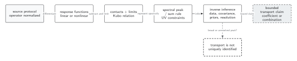
Contact terms, magnetization circulation, conserved overlaps, geometry, and the path to $(\omega,\mathbf k)=(0,0)$ are part of the transport observable. They must be fixed before a Kubo relation is represented spectrally or supplied to an inverse method. The diagram is schematic and does not display boundary-condition or finite-volume details.

In text: differentiate the full source functional, subtract only the local and circulating contributions appropriate to the measurement, retain exact Drude weight, and take volume, regulator, frequency, and momentum limits in the stated order. A different path may define a different physical response.

Exercise: circulation through a cross-section

In three dimensions let $\mathbf J_{\mathrm{mag}}=\boldsymbol\nabla\times\mathbf M$. Show that its flux through an oriented surface $S$ is a boundary current, and state when it vanishes.

Solution

Stokes’ theorem gives

$$\int_S d\mathbf S\cdot\mathbf J_{\mathrm{mag}} =\int_S d\mathbf S\cdot(\boldsymbol\nabla\times\mathbf M) =\oint_{\partial S}\mathbf M\cdot d\boldsymbol\ell.$$

Thus the apparent bulk flux is determined entirely by the boundary. It vanishes for a closed surface, or for a cross-section whose boundary identification and magnetization make the line integral zero. It need not vanish at an open edge or interface, which is why the measurement geometry belongs in the transport definition.

References

• Cooper, Nigel R., Bertrand I. Halperin, and I. M. Ruzin. 1997. “Thermoelectric Response of an Interacting Two-Dimensional Electron Gas in a Quantizing Magnetic Field.” Physical Review B 55 (4): 2344–2359. DOI. Open PDF.
• Kohn, Walter. 1964. “Theory of the Insulating State.” Physical Review 133 (1A): A171–A181. DOI.
• Qin, Tao, Qian Niu, and Junren Shi. 2011. “Energy Magnetization and the Thermal Hall Effect.” Physical Review Letters 107 (23): 236601. DOI. Open PDF.

Spectral Functions and Transport Peaks distinguishes an exact Drude delta function from a broadened relaxation feature. Diffusion, Conductivity, and Susceptibility applies the limit and subtraction rules to coupled transport.