Linearized Kinetics and Relaxation Modes

Linearizing about equilibrium turns the collision kernel into an operator whose null space consists of exact collision invariants. Its nonzero spectrum controls kinetic relaxation. Hydrodynamic modes emerge when streaming perturbs the null space at small wave number; a relaxation-time ansatz that damps those zero modes violates conservation.

Required background. Use collision kernels and detailed balance and spectra, resolvents, and functional calculus.

Helpful background. Memory functions and slow-mode projection gives an operator projection alternative.

Weighted linearized operator

Write

$$f=f_0+f_0(1+\eta f_0)\chi,$$

where $f_0$ is an equilibrium distribution. The homogeneous linearized equation is

$$\partial_t\chi=-\mathcal L\chi.$$

Microreversibility makes $\mathcal L$ symmetric and nonnegative in an equilibrium-weighted inner product; this operator structure is central to the transport calculation of Jeon 1995, §§ II–III. Schematically,

$$\langle\chi_1,\chi_2\rangle =\sum_i\int dP_i\,f_{0i}(1+\eta_if_{0i}) \chi_{1i}\chi_{2i}.$$

For a $2\leftrightarrow2$ reaction,

$$\langle\chi,\mathcal L\chi\rangle \propto\int d\Gamma_{12\leftrightarrow34}\, (\chi_1+\chi_2-\chi_3-\chi_4)^2\ge0.$$

The null vectors are exactly the functions satisfying the additive collision-invariant equation: conserved charges and $p^\mu$. Their completeness depends on the full reaction network.

Hydrodynamic and kinetic sectors

At spatial wave vector $\mathbf k$,

$$\partial_t\chi+\mathbf v\cdot i\mathbf k\,\chi=-\mathcal L\chi.$$

Streaming mixes null and nonnull subspaces. Perturbation theory in $k\ell_{\mathrm{mfp}}$ produces sound, shear diffusion, and charge diffusion from the conserved sector, while nonhydrodynamic eigenvalues remain finite as $k\to0$. A small nonzero collision eigenvalue signals an additional slow variable that may need promotion to hydrodynamics or Hydro+.

The spectrum need not be discrete. Long-range interactions, unbounded momentum space, and angular singularities can produce continuous or accumulating spectra. A finite matrix discretization always returns discrete eigenvalues, so convergence of eigenfunctions, gaps, and weighted observables is essential.

The “H theorem / relaxation modes” box has two related but distinct uses. Linearization studies the spectrum and null space of the collision operator; it does not by itself prove a nonlinear entropy theorem.

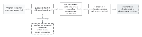
After the equilibrium family and collision measure are fixed, the weighted linearized operator separates exact collision invariants from decaying kinetic modes. Small eigenvalues outside the invariant subspace set long relaxation times and can defeat a proposed closure. The upstream microscopic-matching step can use cuts in a controlled weak-coupling construction. The diagram does not identify this spectral statement with a nonlinear H theorem or guarantee a gap. It is schematic and not to scale.

The sections Weighted linearized operator, Hydrodynamic and kinetic sectors, and Variational transport and missed modes give the text and equation equivalent of the relaxation-mode box.

Checked angular model

Consider elastic angular randomization at fixed $|\mathbf p|$,

$$\partial_t f(\hat{\mathbf p})=-\frac{1}{\tau} \left[f(\hat{\mathbf p})-\frac{1}{4\pi}\int d\Omega' f(\hat{\mathbf p}')\right].$$

Expanding in spherical harmonics gives eigenvalue $0$ for $\ell=0$ and $1/\tau$ for every $\ell\ge1$. The isotropic particle number is conserved while all anisotropies decay. If one replaced the right-hand side by $-f/\tau$, the $\ell=0$ mode would decay incorrectly.

Real collision operators split angular channels and couple energy dependence. The example checks null-space projection, not a quantitative transport time.

Variational transport and missed modes

For a source $S$ orthogonal to the null space, the stationary equation $\mathcal L\chi=S$ can be solved variationally because $\mathcal L\ge0$. Trial spaces give controlled bounds for some transport coefficients when the inner product and operator assumptions hold. If $S$ overlaps a conserved mode, no stationary solution exists until matching conditions remove that component.

A single relaxation time replaces a spectrum by one number. It can match one channel but generally misses momentum dependence, branch cuts, and extra slow modes. Conservation-preserving RTA uses a projector onto the orthogonal complement of the invariant subspace.

Failure tests

• Prove the weighted symmetry or state why the operator is nonnormal.
• Enumerate and numerically recover every collision invariant.
• Refine momentum and angular bases; track spectral pollution and continuous spectra.
• Project sources away from zero modes.
• Compare multiple slow eigenvalues before reducing to one relaxation time.
• Test transport coefficients against direct time evolution.

Exercise

Solve the angular model for initial data $f(\hat{\mathbf p},0)=a+b\cos\theta$.

Solution

$a$ is the $\ell=0$ component and remains constant. $b\cos\theta$ lies in $\ell=1$ and decays as $e^{-t/\tau}$. Hence $f(\hat{\mathbf p},t)=a+b e^{-t/\tau}\cos\theta$.

Continue

Use these modes to motivate moment closures and include unresolved slow internal structure through matrix-valued transport.

References

• Cercignani, C., and Kremer, G. M. (2002). The Relativistic Boltzmann Equation: Theory and Applications. Basel: Birkhäuser. DOI.
• Jeon, S. (1995). “Hydrodynamic Transport Coefficients in Relativistic Scalar Field Theory.” Physical Review D 52, 3591–3642. arXiv:hep-ph/9409250; DOI.