Quasi-de Sitter Validity and Evidence Status

Exact-de Sitter infrared results can be transported to quasi-de Sitter only when background drift, state evolution, coarse-graining, finite duration, and the resummation error are controlled separately. A slowly varying Hubble rate does not guarantee that a long mode has time to relax, and an instantaneous equilibrium density is not generally the solution of a time-dependent Fokker–Planck equation.

Required background. de Sitter infrared regimes fixes the exact-background limits; infrared resummation supplies the dynamical mass; QFT–stochastic matching fixes the observable subset; vacuum choice and initial-state effects supplies finite-time state data; and dynamical renormalization-group resummation supplies an independent secular treatment. Helpful background. Stationary and first-passage observables clarifies duration and boundaries, while relational graviton observables supplies the gauge restriction.

Local transport away from exact de Sitter

For a canonical light spectator, a sharp split, a Bunch–Davies-like short sector, and slowly varying $H(t)$, the leading local cosmic-time model is

$$d\phi_L=-\frac{V'(\phi_L)}{3H(t)}\,dt +\frac{H^{3/2}(t)}{2\pi}\,dW_t, \qquad \mathbb E[dW_t^2]=dt.$$

With $dN=Hdt$, this becomes

$$d\phi_L=-\frac{V'}{3H^2}\,dN +\frac{H}{2\pi}\,dW_N, \qquad \mathbb E[dW_N^2]=dN.$$

The displayed coefficients are a leading local approximation, not an identity for every inflaton or gauge. Mass, sound speed, slow parameters, the time-dependent window, and the transformation between the gauge used for short-mode quantization and the stochastic clock produce calculable corrections.

For a free massless spectator, the local model predicts

$$\sigma^2(N)-\sigma^2(0) =\int_0^N\frac{H^2(n)}{4\pi^2}\,dn.$$

If $\epsilon_H=-d\ln H/dN$ is constant, $H=H_0e^{-\epsilon_HN}$ and

$$\sigma^2(N)-\sigma^2(0) =\frac{H_0^2}{8\pi^2\epsilon_H} \left(1-e^{-2\epsilon_HN}\right) =\frac{H_0^2}{4\pi^2} \left(N-\epsilon_HN^2+\cdots\right).$$

The $\epsilon_HN^2$ term is a background-drift correction. Failure of a secular expansion at very large $N$, by contrast, is a duration or resummation problem. Combining them into a single unspecified “slow-roll error” hides which approximation failed.

First application: transporting a dynamical mass

Use the large-N quartic convention $V=\lambda(\boldsymbol\phi^2)^2/(4!N_f)$. In exact de Sitter, the massless stationary gap equations give

$$M_{\rm dS}^2=\frac{\sqrt\lambda}{4\pi}H^2, \qquad F_{\rm eq}=\frac{3H^2}{2\pi\sqrt\lambda}.$$

A local quasi-de Sitter transport ansatz replaces $H$ by $H(N)$ in the gap while evolving the variance rather than setting it instantly to $F_{\rm eq}(N)$:

$$\frac{dF}{dN} =\frac{H^2(N)}{4\pi^2} -\frac{2M_{\mathrm{loc}}^2(N)}{3H^2(N)}F,$$ $$F(N)=e^{-I(N)} \left[ F(0)+\int_0^N e^{I(n)}\frac{H^2(n)}{4\pi^2}\,dn \right], \qquad I(N)=\int_0^N\frac{2M_{\mathrm{loc}}^2}{3H^2}\,dn.$$

For the local large-N mass, the relaxation gap in e-fold time is $\sqrt\lambda/(6\pi)$. Adiabatic tracking requires

$$\left\lvert\frac{d\ln F_{\rm eq}}{dN}\right\rvert \ll\frac{\sqrt\lambda}{6\pi};$$

for constant $\epsilon_H$, this means $2\epsilon_H\ll\sqrt\lambda/(6\pi)$. If the inequality fails or inflation lasts fewer than roughly $6\pi/\sqrt\lambda$ e-folds, the finite-time integral is the prediction; the exact-de Sitter equilibrium value is not reached. Corrections from finite $N_f$, the resummation scheme, the window, and slow variation must be quoted independently.

The theoretical status beyond slow roll is formulation-sensitive. A separate-universe and gauge analysis finds controlled noise corrections in several slow-roll and ultra-slow-roll examples Pattison et al. 2019, §§2–7, Eqs. (2.15)–(7.12), whereas a different truncation analysis identifies regimes where the traditional stochastic treatment fails beyond leading slow-roll order Cruces, Germani, and Prokopec 2019, §§2–4, pp. 2–13. These are model and formalism results, not a universal theorem in either direction. A 2026 open-system construction derives a Lindblad description and a diagonal Fokker–Planck limit including specified deviations from exact de Sitter Li 2026, main-text Eqs. (13)–(21) and Supplemental §§4–5, but its zero-mode and truncation assumptions still delimit the result.

The structure map treats quasi-de Sitter evolution as a transport problem with independent state, drift, window, relaxation, and matching inputs.

Local exact-de Sitter data can seed finite-time transport only when slow background drift is smaller than the relevant relaxation and matching scales. Schematic; not to scale.

Domain, evidence, and failure conditions

Use the chapter’s canonical domain table. The evidence statement here is current through 10 August 2026. The worked transport concerns a light spectator and a local slow-variation expansion; inflaton fluctuations require the constraints, a clock choice, and a gauge-consistent noise calculation. Tensor claims still require relational observables. No observational parameter value is inferred here.

Adversarial test. Recompute the same finite-time scalar variance with an in-in or dynamical-RG treatment, translate state and renormalization conventions, and vary the coarse-graining window. Separately vary $\epsilon_H$, total duration, initial state, and resummation method. Demand convergence in a joint regime where slow drift, window dependence, and omitted secular terms are each small. Search for contrary calculations that treat the same observable and approximation order; apparent disagreement in a different gauge or with an instantaneous-equilibrium substitution is not yet a contradiction.

The failure map rejects an exact-de Sitter equilibrium inserted into a background that evolves faster than its relaxation gap, a formally small slow parameter multiplied by an uncontrolled duration, and a stochastic scalar result promoted to a gauge-invariant gravitational claim. Outside the overlap regime, return to QFT–stochastic matching, open-system dynamics, or relational graviton observables rather than extending the local formula.

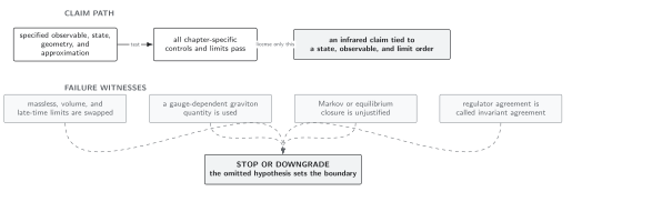
Background drift, finite duration, state preparation, coarse-graining, resummation, and observable definition require separate error estimates. Schematic; not to scale.

References

• Cruces, D., C. Germani, and T. Prokopec, “Failure of the Stochastic Approach to Inflation Beyond Slow-Roll,” Journal of Cosmology and Astroparticle Physics 2019(03), 048 (2019), doi:10.1088/1475-7516/2019/03/048.
• Li, Y.-Z., “Stochastic Inflation as an Open Quantum System,” Physical Review Letters 136, 071501 (2026), doi:10.1103/hlfz-8lhg.
• Pattison, C., V. Vennin, H. Assadullahi, and D. Wands, “Stochastic Inflation Beyond Slow Roll,” Journal of Cosmology and Astroparticle Physics 2019(07), 031 (2019), doi:10.1088/1475-7516/2019/07/031.