From Propagators and Response Functions to Channel Maps

Localized couplings turn curved-space Green functions and field covariances into an input–output map. The causal propagator determines how a sender displacement reaches the receiver; the state-dependent symmetric two-point function determines fluctuations. Keeping these kernels separate yields a Gaussian channel in linear models and prevents vacuum correlations from being misidentified as transmission.

Required background. Green Operators, Causal Propagators, and State-Dependent Two-Point Functions fixes $E=G_{\mathrm{ret}}-G_{\mathrm{adv}}$. Curved-Spacetime Channel Deployment Contract fixes the operational data. Communication Through Quantum Fields supplies the sender–field–receiver construction.

Helpful background. Wavepackets, Modes, Frames, and Localization controls mode normalization. Scalar Propagators, Ordered Correlators, and Sources compares retarded, Wightman, and ordered kernels.

Response and fluctuation kernels

For linear observables $\Phi(f)$ and $\Phi(h)$, define

$$E(f,h)=\int_{M\times M}f(x)E(x,x')h(x') \,d\mathrm{vol}_g(x)d\mathrm{vol}_g(x')$$

and

$$H_\omega(f,h)=\frac12\,\omega\!\left( \{\Phi(f),\Phi(h)\}\right).$$

The site convention gives $[\Phi(f),\Phi(h)]=-iE(f,h)$. Linear response of an observable supported later than a source is therefore controlled by the retarded part of $E$, up to the sign fixed by the interaction Hamiltonian. By contrast, $H_\omega$ is a positive covariance that depends on the state. The Wightman function combines them,

$$\omega_2(f,h)=H_\omega(f,h)-\frac{i}{2}E(f,h),$$

for real smearings. Using $\omega_2$ wholesale as a signal kernel would make the putative gain state dependent and generally nonzero for spacelike-separated supports.

Linear probes and the Gaussian channel

Let $R_A=(q_A,p_A)^T$ and $R_B=(q_B,p_B)^T$ be oscillator quadratures. Linear probe–field evolution is symplectic on the combined probe and field phase space. After tracing the field and the receiver’s initial state, the sender-to-receiver reduced map has

$$d_B^{\mathrm{out}}=X,d_A^{\mathrm{in}}+d_0, \qquad V_B^{\mathrm{out}}=X V_A^{\mathrm{in}}X^T+Y.$$

Here $d$ is the first-moment vector and $V_{jk}=\langle\{R_j-d_j,R_k-d_k\}\rangle/2$. For a physical one-mode Gaussian channel,

$$Y+\frac{i}{2}\left(\Omega_B-X\Omega_A X^T\right)\ge0, \qquad \Omega=\begin{pmatrix}0&1\\-1&0\end{pmatrix}.$$

This complete-positivity inequality is an independent check on any perturbatively assembled $X$ and $Y$.

Suppose the sender couples first and the receiver second through smooth spacetime smearings $f_A$ and $f_B$. To leading nontrivial order, each entry of $X$ is a detector-response-weighted version of

$$\mathcal G_{BA} =\lambda_A\lambda_B \int d\tau_Bd\tau_A\, \chi_B(\tau_B)\chi_A(\tau_A) r_B(\tau_B)r_A(\tau_A) G_{\mathrm{ret}}\!\left(z_B(\tau_B),z_A(\tau_A)\right),$$

with the spatial smearings understood. The functions $r_\nu$ are the appropriate free probe response factors. The added covariance $Y$ contains the receiver’s initial covariance, local noise, and integrals of $H_\omega$. Exact linear detector–field models have the same structural division, even when perturbation theory is unnecessary; a concrete oscillator realization is given by Lapponi et al. 2023, §§ II–III.

Sequential stationary application

On a stationary globally hyperbolic spacetime, choose a stationary quasifree Hadamard state and two normalized spatial smearings transported along stationary worldlines. Let $A$ interact during $[t_0,t_1]$ and $B$ during $[t_2,t_3]$ with $t_2>t_1$. The free probe evolution matrices $S_A(t)$ and $S_B(t)$ supply the sine and cosine response factors. Then

$$X_{BA}^{(2)} =\lambda_A\lambda_B \int_{t_2}^{t_3}\!dt \int_{t_0}^{t_1}\!dt'\, S_B(t_3-t)\,C_B\, G_{\mathrm{ret}}^{BA}(t,t')\, C_A^T S_A(t'-t_0),$$

where $C_A,C_B$ select the coupled quadratures and $G_{\mathrm{ret}}^{BA}$ is the spatially smeared retarded kernel. At the same order, $Y$ is built from double integrals of $H_\omega^{BB}$ together with the propagated initial $B$ covariance. Retaining the full block symplectic evolution automatically adds the terms needed for complete positivity; truncating $X$ and $Y$ inconsistently may violate it.

Three checks make this calculation reproducible:

• $X_{BA}=0$ whenever the sender support is outside the causal past of the receiver support.
• The state can change $Y$ while $X_{BA}$ remains fixed for a free field with fixed geometry and couplings.
• In the flat stationary limit, the result reduces to the corresponding Minkowski detector channel.

This is the requested leading Gaussian channel: $X$ is the causal transfer matrix and $Y$ is the declared added covariance.

Replacing response by a Wightman function

Perform the adversarial substitution $G_{\mathrm{ret}}^{BA}\mapsto\omega_2^{BA}$. For spacelike-separated supports, $G_{\mathrm{ret}}^{BA}=0$ but $\omega_2^{BA}$ is generally nonzero. The resulting “gain” would allow the sender’s choice to change the receiver output outside causal contact. What survives is a statement about joint fluctuations or correlation extraction, not a sender-to-receiver channel. The decisive repair is to restore the commutator/retarded kernel in $X$ and retain the symmetric covariance only in $Y$ or in joint detector correlations.

Domain, limits, and maps

See the canonical Domain and failure conditions. The formulas above assume a free field, linear probes, specified smearings, and either controlled weak coupling or an exact quadratic model. Interacting fields, nonlinear detectors, time-dependent backgrounds, or repeated uses with memory require a more general channel construction. A Gaussian fit does not prove that neglected cumulants vanish.

The structure map highlights the transition from propagation to receiver restriction. Inspect the checkpoint below it: commutator support validates $X$, while state covariance and frame transformations enter different parts of the map.

For linear probes, causal propagation determines the transfer matrix $X$ and state fluctuations contribute to $Y$ before receiver restriction and decoding. Schematic; not to scale.

The failure map’s correlation witness is realized by the Wightman substitution. It produces a correlation calculation but does not license a causal channel map.

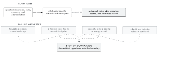
State-dependent two-point correlations cannot replace the retarded response in a signaling matrix; spacelike support exposes the error. Schematic; not to scale.

Handoffs

Causal Support, Signaling, and Global Geometry studies the support of $X$. Redshift, Restricted Access, and Effective Channel Noise separates unitary mode conversion from reduction to an effective channel. Abstract Gaussian-channel capacities belong to Energy-Constrained Capacities and Coding Tasks.

References

• Barcellos, Ian Bernardes, and André G. S. Landulfo. “Relativistic Quantum Broadcast Channel.” Physical Review D 109 (2024): 065020. DOI. Open PDF.
• Lapponi, Alessio, Dimitris Moustos, David Edward Bruschi, and Stefano Mancini. “Relativistic Quantum Communication between Harmonic Oscillator Detectors.” Physical Review D 107 (2023): 125010. DOI. Open PDF.