Causal, Killing, Trapping, and Apparent Horizons: The QFT Interface

Different horizons answer different geometric questions. An event horizon is defined using the entire causal future, a Killing horizon uses a symmetry generator, a trapping or apparent horizon uses null expansions on chosen surfaces, and an acceleration horizon is observer dependent. A QFT calculation is sound only when it requests the structure that its state, mode, detector, or flux construction actually uses.

Required background. Curved spacetimes and global hyperbolicity supplies Cauchy evolution and causal futures.

Helpful background. Levi–Civita connections and curvature fixes the null-geometric conventions, and causal support and signaling relates global causal regions to observables.

Horizon classes and their QFT data

For an asymptotically predictable spacetime with future null infinity $\mathscr I^+$, the future event horizon is

$$\mathcal H^+=\partial J^-(\mathscr I^+).$$

This is a global, teleological definition: deciding whether an event lies inside requires knowledge of the entire future. More generally, the causal horizon of a worldline or region is the boundary of its causal past. Rindler and de Sitter static-patch horizons fit this observer- or region-relative definition without being black-hole event horizons.

A Killing horizon is a null hypersurface to which a Killing field $\chi$ is normal. It supplies a conserved Killing frequency and, when nondegenerate, surface gravity. A bifurcate Killing horizon has a codimension-two surface where $\chi=0$ and is the natural setting for many horizon-regular KMS theorems. Neither stationarity nor a bifurcation surface follows from the existence of a general event horizon.

For a spacelike two-surface $S$ with future null normals $\ell^\mu$ and $n^\mu$, the expansions are

$$\theta_{(\ell)}=q^{\mu\nu}\nabla_\mu\ell_\nu, \qquad \theta_{(n)}=q^{\mu\nu}\nabla_\mu n_\nu.$$

A marginally outer trapped surface has $\theta_{(\ell)}=0$ and usually $\theta_{(n)}<0$. A future outer trapping horizon is a hypersurface foliated by such surfaces with an additional outer condition, commonly $\mathcal L_n\theta_{(\ell)}<0$ after fixing orientations. An apparent horizon is the outer boundary of trapped surfaces on a chosen slice and can change with the foliation. These quasi-local notions are valuable in dynamical geometry, but they do not automatically supply a Killing frequency or a global in/out mode basis. The distinction and its dynamical uses are reviewed in Ashtekar and Krishnan 2004, §§ 2–3.

QFT task	Minimum geometric structure
Define a stationary KMS frequency	Timelike Killing flow in the region and its horizon generator
Derive collapse ray peeling	A regular affine null coordinate and a late-time null map; a globally known event horizon is sufficient but not the only useful formulation
Test horizon regularity of a two-point function	Regular coordinates across the relevant null horizon and a Hadamard condition
Compute greybody transmission	A separable or otherwise well-posed scattering problem with asymptotic boundary conditions
Predict a local detector response	Detector worldline, switching, state two-point function, and causal domain; an event horizon is not by itself required

The structure map begins with this classification because all later arrows depend on it. Inspect the first box: replacing one horizon by another changes the available generator, state domain, or causal boundary data before any thermal calculation starts.

Geometric entry point to a Hawking-radiation calculation. The diagram is schematic and not to scale; causal, Killing, trapping, and observer horizons supply different downstream data.

The failure map names the page’s adversarial test directly. Interchanging horizon classes does not merely change terminology: it can remove the symmetry, global boundary, or observer specification used in the derivation.

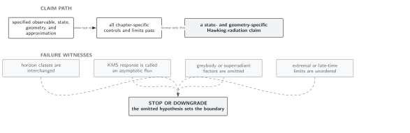
Failure boundary for horizon classification. This schematic, not-to-scale map downgrades the claim to the geometric structure actually verified rather than transferring a thermal or flux result unchanged.

Application: Schwarzschild and collapse

In the maximally extended Schwarzschild geometry, the surface $r=2M$ is an event horizon and a Killing horizon of the asymptotically normalized $\partial_t$; the extension contains a bifurcation sphere. On standard symmetric slices, the marginal surface also lies at $r=2M$. These coincidences are special to stationarity and symmetry.

During spherical collapse, the event horizon is still $\partial J^-(\mathscr I^+)$ and can extend into a region before any local trapped surface appears. Marginally trapped tubes depend on the evolving matter and slicing. There is generally no exact Killing generator during collapse, although the exterior may approach Schwarzschild at late retarded time. The Hawking collapse calculation therefore uses a regular early affine coordinate, causal propagation, and the late-time exponential null map. It must not assume an exact global KMS state during the dynamical phase.

For an acceleration horizon in Minkowski spacetime, a uniformly accelerated detector can show KMS detailed balance with respect to boost time, while inertial future null infinity has no black-hole luminosity. Substituting this observer horizon for a collapse event horizon preserves the local near-horizon kinematics but removes the state preparation and asymptotic flux claim.

Domain and failure conditions

The canonical distinctions are in the chapter domain and failure-conditions table. This page licenses only the QFT structures listed for the horizon class actually established. The decisive checks are the defining causal boundary, null expansions and foliation, or Killing normality and normalization. If an event horizon is replaced by an apparent horizon, global in/out claims must be dropped; if a Killing horizon is replaced by a generic causal horizon, KMS frequency and surface-gravity claims must be dropped. The valid handoff is the precise geometric data that remain.

Exercise

Explain why locating $\theta_{(\ell)}=0$ on one slice cannot by itself determine a Hawking temperature.

Solution

The equation identifies a marginal surface relative to chosen null normals and slicing. A Hawking temperature requires a normalized time flow or a collapse peeling rate. A generic marginal surface supplies neither a Killing generator nor an affine-to-retarded-time exponential map. Additional stationarity or dynamical assumptions are therefore necessary.

Handoff

When a nonextremal stationary Killing horizon is available, its normalized generator fixes surface gravity, redshift, and the exponential relation between Killing and affine null parameters.

References

• Ashtekar, Abhay, and Badri Krishnan. “Isolated and Dynamical Horizons and Their Applications.” Living Reviews in Relativity 7 (2004): 10. doi:10.12942/lrr-2004-10.
• Kay, Bernard S., and Robert M. Wald. “Theorems on the Uniqueness and Thermal Properties of Stationary, Nonsingular, Quasifree States on Spacetimes with a Bifurcate Killing Horizon.” Physics Reports 207 (1991): 49–136. doi:10.1016/0370-1573(91)90015-E.
• Wald, Robert M. General Relativity. Chicago: University of Chicago Press, 1984. Publisher record.