Quantum Energy Inequalities in Curved Spacetime

A quantum energy inequality (QEI) bounds how negative a renormalized energy density can remain after smooth sampling, for a specified field, state class, curve, and stress prescription. The most robust curved-spacetime results are timelike worldline inequalities for free fields in Hadamard states. They do not imply pointwise positivity and cannot generally be converted into a four-dimensional null-worldline bound by boosting the observer.

Required background. Classical energy conditions and quantum violations supplies the pointwise contrast; quantum energy inequalities supplies the abstract bound; and the Hadamard parametrix supplies ultraviolet admissibility.

Helpful background. Renormalized stress-tensor ambiguities fixes finite local shifts, while test functions and distributions explains why the sampler must be smooth.

Timelike worldline inequalities

Let $\gamma(\tau)$ be a smooth timelike curve parametrized by proper time, with unit tangent $u^\mu$, and let $g\in C_0^\infty(\mathbb R)$ be real. A QEI has the form

$$\int_{-\infty}^{\infty}d\tau\, g(\tau)^2 \langle T_{\mu\nu}u^\mu u^\nu\rangle_{\omega,\mathrm{ren}} \ge-\mathcal B[g,\gamma,\mathcal G,m,\xi],$$

for every state $\omega$ in the theorem’s class. Here $\mathcal G$ denotes the local geometric and renormalization data. An absolute QEI has a right-hand side determined by geometry and field parameters; a difference QEI bounds the stress relative to a specified reference Hadamard state. These are distinct statements.

For a minimally coupled scalar on a four-dimensional globally hyperbolic spacetime, Fewster and Smith establish an absolute curved-spacetime QEI using the local Hadamard expansion (Fewster and Smith 2008, Theorem 3.1). Its explicit bound involves the pullback of a locally constructed bidistribution and geometric correction terms. The theorem does not cover arbitrary interactions, non-Hadamard states, or nonsmooth switching.

In four-dimensional Minkowski spacetime, for a massless scalar and inertial $\gamma$,

$$\int d\tau\,g(\tau)^2\langle T_{uu}\rangle_\omega \ge-\frac{1}{16\pi^2} \int d\tau\,\lvert g''(\tau)\rvert^2.$$

This normalization uses the weight $g^2$. Writing a theorem with a sampler $f=g^2$ changes the apparent derivative structure and requires $f$ to admit the needed smooth square root.

The structure map shows that “QEI” becomes a usable statement only after the timelike curve, proper-time sampler, state class, field, dimension, and subtraction data have been supplied.

Inputs to a curved timelike QEI. The map is schematic and not to scale; the lower bound is a functional of the sampler and local geometry, not a universal constant or pointwise floor.

Static curved region and the short-sampling limit

Choose a geodesic segment inside a static region with curvature radius $L_R$, distance $L_B$ from any boundary, and a compact sampler

$$g_{\tau_0}(\tau) =\tau_0^{-1/2}g_1(\tau/\tau_0), \qquad \int d\tau\,g_{\tau_0}^2=1.$$

For the flat massless bound,

$$\mathcal B_{\mathrm{flat}}[g_{\tau_0}] =\frac{1}{16\pi^2\tau_0^4} \int ds\,\lvert g_1''(s)\rvert^2.$$

The $\tau_0^{-4}$ scaling is both dimensional and operational: shorter measurements permit more negative averaged energy. In a static curved region, a local expansion has the schematic hierarchy

$$\mathcal B =\mathcal B_{\mathrm{flat}} \left[ 1+O(m^2\tau_0^2) +O(\lvert R\rvert\tau_0^2) +O(a_{\mathrm{obs}}^2\tau_0^2) +O(\tau_0^2/L_B^2) \right],$$

where the displayed form means relative corrections in a regime where all ratios are small; coefficients depend on the field, coupling, curve, and sampler. One must use the actual curved theorem rather than this expansion when $\tau_0$ approaches any geometric scale.

The application is reproducible by stating $g_1$, its width convention, $m$, $\xi$, the worldline, curvature invariants over the sampler support, reference state if any, and finite stress prescription. The decisive flat check is

$$\lim_{\tau_0/L_R\to0} \tau_0^4\mathcal B[g_{\tau_0}] =\frac{1}{16\pi^2} \int ds\,\lvert g_1''(s)\rvert^2.$$

Why the null limit fails

Boosting the timelike observer while holding a coordinate-time sampler fixed changes its proper-time width and the stress projection simultaneously. The limit is not uniform. In four-dimensional Minkowski QFT, Fewster and Roman construct states showing that no nontrivial state-independent null-worldline QEI of the analogous form exists (Fewster and Roman 2003, §§ II–III). ANEC can still hold because its complete, unsmeared null integral is a different limit with different hypotheses.

The adversarial cases are immediate:

• a non-Hadamard two-point function makes the local stress or theorem’s wavefront products inadmissible;
• a top-hat sampler has distributional derivatives and lies outside the smooth theorem;
• $\tau_0\sim L_R$ invalidates the short-sampling expansion; and
• taking a null boost while silently holding the wrong width fixed does not prove a null QEI.

The failure map locates these as domain failures, not small corrections to the same bound.

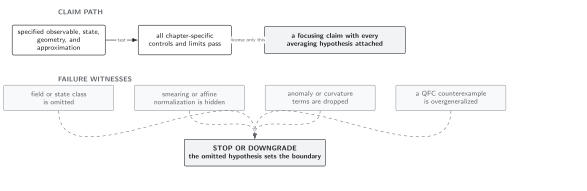
Failure modes of a timelike worldline QEI. The diagram is schematic and not to scale; a failed sampler or state hypothesis withdraws the theorem, while a long sampling time requires the full curved bound rather than its local flat limit.

Domain and failure conditions

See the chapter domain and failure-conditions table. The explicit application concerns a free scalar, Hadamard states, a smooth compact proper-time sampler, and a timelike curve in a controlled static region. It does not establish a general interacting QEI, a boundary theorem, a pointwise bound, or a four-dimensional null-worldline inequality.

Exercise

Show that the flat bound scales as $\tau_0^{-4}$ under $g_{\tau_0}(\tau)=\tau_0^{-1/2}g_1(\tau/\tau_0)$.

Solution

Two derivatives give $g_{\tau_0}''=\tau_0^{-5/2}g_1''(\tau/\tau_0)$. Hence

$$\int d\tau\,\lvert g_{\tau_0}''\rvert^2 =\tau_0^{-5}\int d\tau\, \lvert g_1''(\tau/\tau_0)\rvert^2 =\tau_0^{-4}\int ds\,\lvert g_1''(s)\rvert^2.$$

References

• Fewster, C. J., and S. P. Eveson. “Bounds on Negative Energy Densities in Flat Spacetime.” Physical Review D 58 (1998): 084010. DOI.
• Fewster, C. J., and T. A. Roman. “Null Energy Conditions in Quantum Field Theory.” Physical Review D 67 (2003): 044003; erratum 80 (2009): 069903. DOI.
• Fewster, C. J., and C. J. Smith. “Absolute Quantum Energy Inequalities in Curved Spacetime.” Annales Henri Poincaré 9 (2008): 425–455. DOI.