Cosmological Loops and Renormalization

Cosmological loop calculations combine ultraviolet renormalization with state dependence, infrared sensitivity, and long-time evolution. These are different problems. A covariant ultraviolet pole is removed by local bulk, boundary, and composite-operator counterterms; an infrared or secular logarithm is controlled by the physical volume, mass, duration, observable, and initial state.

Required background. In-in cosmological correlators supplies the doubled perturbation theory; contours and initial boundaries supplies state counterterms; the EFT of inflation supplies power counting; and counterterms, subdivergences, and locality supplies the ultraviolet theorem.

Helpful background. Interacting curved-spacetime correlators supplies local covariant products; renormalized contact products supplies coincident insertions; and cubic interactions and bispectra supplies the tree normalization.

Ultraviolet subtraction on the closed time path

Regulate the spatial and time integrals in a way that preserves as much covariance and contour structure as possible. In dimensional regularization the divergent effective action has the local form

$$\Gamma_{\rm div}=\frac1{d-4} \int d^4x\sqrt{-g}\sum_i c_i\mathcal O_i[g,\phi] +\Gamma_{\rm boundary,div},$$

where $\mathcal O_i$ includes every operator allowed by the EFT symmetries at the relevant order. Expanding these counterterms about FLRW generates counterterm vertices for $\zeta$ and $\gamma$. A renormalized spectrum therefore has the schematic organization

$$\mathcal P_\zeta^{\rm ren}(k,t)= \mathcal P_\zeta^{\rm tree}(k,t) +\mathcal P_\zeta^{\rm loop}(k,t;\mu) +\sum_i C_i(\mu)\mathcal P_{\zeta,i}^{\rm local}(k,t).$$

Renormalization-group invariance requires the explicit $\mu$ dependence to cancel the running of $C_i$ to the computed order. Power divergences or cutoff-dependent terms cannot be interpreted before matching the regulator to this local operator basis.

The one-loop organization for inflationary two-point functions, including the need for local counterterms and late-time definitions, is developed in Senatore and Zaldarriaga 2010, §§2–4, Eqs. (12)–(74).

Ultraviolet, infrared, and time logarithms

Three symbols that look like logarithms answer different questions:

$$\ln\frac{k}{\mu}, \qquad \ln(kL), \qquad N(t,t_0)=\ln\frac{a(t)}{a(t_0)}.$$

The first accompanies ultraviolet running; the second can encode sensitivity to an infrared box or long-mode definition; the third measures elapsed expansion and can signal nonuniform late-time perturbation theory. Their coefficients can mix in intermediate formulas, but a controlled calculation varies $\mu$, $L$, and $t_0$ independently. Gauge or composite observables may eliminate some apparent infrared dependence.

For the first application, renormalize a one-loop quasi-de Sitter scalar two-point function. Isolate $1/(d-4)$ poles and cancel them with local operators, verify $\mu$ independence, then study the finite result as the infrared regulator and observation time vary. Report a secular coefficient only after it survives ultraviolet scheme changes and the observable has been fixed. Weinberg proves bounds on late-time growth for a broad class of interactions in Weinberg 2006, §§II–IV, Eqs. (7)–(35); those bounds do not assert that every logarithm is physical.

Subdivergences provide a stringent internal check. Counterterm insertions determined at lower loop order must cancel every nested UV pole before the overall divergence is removed. On the closed time path the same renormalized coefficient appears on both branches with opposite action signs; inventing independent $+$ and $-$ bulk couplings would violate unitarity. Boundary-state and composite-operator coefficients are additional parameters, but their branch structure is likewise constrained by Hermiticity and normalization.

The structure map separates renormalization from the subsequent infrared and secular analysis.

Ultraviolet locality, boundary-state renormalization, infrared regulation, and secular evolution are distinct parts of a cosmological loop calculation and require independent controls. Schematic; not to scale.

Independent-regulator adversarial test

Change the ultraviolet scheme while holding the renormalized Wilson coefficients fixed at one matching scale. The nonlocal finite prediction must agree. Next change only the infrared regulator or finite observation region; any variation must be assigned to the observable definition or physical long-mode sensitivity. Finally vary $t_0$ with the state action run consistently. A claimed secular coefficient that changes under a purely ultraviolet finite counterterm is not yet a scheme-independent observable.

Composite late-time fields can require their own local renormalization, and a gauge-fixed correlator can carry removable long-distance growth. See the chapter’s domain and failure conditions.

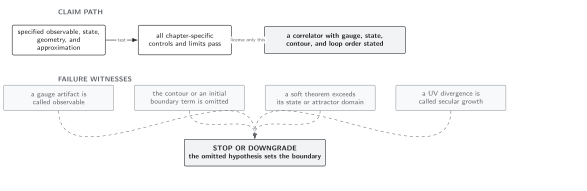
A loop result is accepted only after local UV subtraction, state and composite renormalization, and independent IR and duration variations identify which logarithms belong to the declared observable. Schematic; not to scale.

References

• Senatore, L., and M. Zaldarriaga, “On Loops in Inflation,” Journal of High Energy Physics 12, 008 (2010), doi:10.1007/JHEP12(2010)008.
• Weinberg, S., “Quantum Contributions to Cosmological Correlations. II. Can These Corrections Become Large?” Physical Review D 74, 023508 (2006), doi:10.1103/PhysRevD.74.023508.