Constraint Solving and the Gauge-Observable Ledger

An inflationary calculation passes through several kinds of variable: lapse and shift enforce constraints, a gauge choice selects representatives, field redefinitions simplify the action, and the final late-time field is only a proxy for an observable under stated assumptions. Keeping this dictionary explicit prevents a gauge-fixed cubic vertex from being mistaken for a gauge-independent prediction.

Required background. Gauge-invariant perturbations supplies the transformation rules; Mukhanov–Sasaki scalar modes supplies the reduced scalar variable; and tensor modes fixes the transverse-traceless sector.

Helpful background. Relational gravitational observables supplies an operational completion, while gauge, BRST, and BV methods on curved backgrounds supplies the systematic quantum treatment of gauge redundancy.

From ADM variables to a reduced action

In comoving gauge,

$$N=1+\alpha,\qquad N_i=\partial_i\beta+N_i^T,\qquad h_{ij}=a^2e^{2\zeta}(e^\gamma)_{ij},$$

with $\partial_iN_i^T=0$, $\partial_i\gamma_{ij}=0$, and $\gamma_{ii}=0$. The lapse perturbation $\alpha$ and shift components have no independent propagating initial data in the two-derivative theory. At linear scalar order their equations give, schematically,

$$\alpha=\frac{\dot\zeta}{H}, \qquad \partial^2\beta=a^2\epsilon\dot\zeta+\text{local terms fixed by convention}.$$

The precise decomposition of $\beta$ differs between authors because a local $-\zeta/H$ term may be separated before defining the inverse-Laplacian variable. The invariant procedure is to vary the unreduced ADM action, solve with declared boundary conditions, and substitute the solution back. Substituting a guessed constraint solution before variation can lose equations or boundary contributions.

At quadratic order this reduction yields

$$S_2=M_{\rm Pl}^2\int dt\,d^3x\,a^3\epsilon \left[\dot\zeta^2-\frac{(\partial_i\zeta)^2}{a^2}\right].$$

At cubic order the same constraints generate nonlocal-looking inverse Laplacians whose final correlators are local in the EFT sense. Maldacena’s complete reduction, including endpoint terms and terms proportional to the linear equation of motion, is given in Maldacena 2003, §3, Eqs. (3.1)–(3.15).

Field maps and the late-time quantity

A term in the cubic action of the form

$$S_3\supset\int d^4x\,F(\zeta)\frac{\delta S_2}{\delta\zeta}$$

can be removed perturbatively by $\zeta=\zeta_n+F(\zeta_n)$. This does not erase its contribution: the nonlinear map itself contributes to $\langle\zeta\zeta\zeta\rangle$. Likewise, an integration by parts shifts bulk interactions into initial or final boundary terms. They may be dropped only if the state, contour, and external-time prescription make their contribution vanish or if they are included through the transformed wavefunctional.

The first application is the scalar three-point function. Starting from the ADM action, solve $N$ and $N_i$ through the order needed, reduce to $\zeta$, remove equation-of-motion terms with a declared field redefinition, compute on the in-in contour, and take the late-time limit. The observable dictionary is

$$(N,N_i,h_{ij},\phi) \longrightarrow (\zeta,\gamma_{ij})_{\rm gauge} \longrightarrow (\zeta_n,\gamma_{ij})_{\rm canonical} \longrightarrow \zeta_{\rm late} \longrightarrow \text{declared relational or observational proxy}.$$

Each arrow has a domain: the last one assumes an attractor and subsequent transfer physics that preserves or predictably evolves $\zeta$.

At nonlinear order, even the phrase “late $\zeta$” needs a prescription. One may define it as the perturbation of the integrated expansion between an initial flat slice and a final uniform-density slice, or as the scalar part of a relationally selected spatial metric. These agree in the separate-universe attractor regime but can differ when gradients, entropy transfer, or the clock slicing matter. Declaring that definition before comparing gauges prevents an unnoticed change of target.

The structure map makes these translations explicit before the correlator is interpreted.

Constraint variables, gauge representatives, canonical fields, late-time proxies, and relational observables are connected by calculable but assumption-dependent maps. Schematic; not to scale.

Two-gauge adversarial check

Repeat the same three-point calculation in comoving gauge and in a spatially flat or Goldstone gauge. Retain the Gibbons–Hawking–York contribution where relevant, all temporal endpoints, constraint-induced terms, and the nonlinear map between fields. The two answers must agree after translating the final observable. A mismatch localized to a polynomial momentum term often signals a contact or boundary convention; a mismatch in a nonanalytic momentum dependence signals a physical or algebraic error.

The chapter’s domain and failure conditions compare this check with state and EFT checks. The validity map shows why solving constraints without tracking the observable map is insufficient.

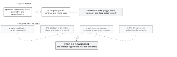
A reduced correlator is accepted only after two complete gauges agree, including constraints, endpoints, field redefinitions, and the same late-time observable. Schematic; not to scale.

References

• Maldacena, J., “Non-Gaussian Features of Primordial Fluctuations in Single Field Inflationary Models,” Journal of High Energy Physics 05, 013 (2003), doi:10.1088/1126-6708/2003/05/013.