

Negative Energy and Quantum Interest
Quantum interest is the statement that a negative-energy episode allowed by a QEI must be compensated by positive energy, with the required compensation depending on duration and separation. It is not a universal pulse law: the result inherits the field, dimension, state class, worldline, sampler family, geometry, and smoothness assumptions of the underlying QEI. A clean formulation turns the bound into a variational problem for two smooth pulses.
Required background. Curved-spacetime QEIs supplies the worldline bound; quantum energy inequalities supplies its operator interpretation; and quantum interest supplies the compensation question.
Helpful background. ANEC gives a distinct null average, while Casimir effects illustrates stationary negative energy that is not an isolated timelike pulse.
Two smooth timelike pulses
Section titled “Two smooth timelike pulses”Along an inertial proper-time worldline, take
where , , and
Thus are the signed pulse areas in the chosen proper-time normalization. Applying a QEI with weight gives
where
For every admissible with ,
The strongest lower bound furnished by that QEI is therefore
This formula is already a reproducible determination of the minimum: specify the QEI, pulse shape, and function space, then converge the variational supremum. Calling the “interest” is useful only when the optimized result actually enforces .
The structure map places compensation after the timelike QEI and its complete sampler/state data, not after a pointwise negative measurement alone.

Quantum-interest variational problem. The map is schematic and not to scale; pulse areas, widths, separation, proper-time normalization, field, state class, and geometry all enter the compensation threshold.
Fourth-order operator test in four dimensions
Section titled “Fourth-order operator test in four dimensions”For the massless scalar inertial QEI,
for all real smooth compact . After integration by parts, this is positivity of the quadratic form of
For fixed , , and , increase until the lowest eigenvalue or infimum of this form reaches zero. That threshold is the QEI-allowed minimum for the chosen pulse model. Numerical reproduction requires a domain much larger than , boundary-condition variation, basis or mesh refinement, and recovery of the zero-pulse spectrum.
Two limits check the result:
- as with identical pulse shapes, the stress tends to , so a nonnegative net pulse is sufficient;
- as the negative pulse narrows at fixed , high derivatives of optimizing samplers become expensive, restricting the amount and duration of negative energy.
Ford and Roman formulate the quantum-interest conjecture and analyze pulse separation and overcompensation in representative QEI models (Ford and Roman 1999, §§ II–IV). The exact threshold is not transferable between dimensions or fields because the differential order and bound kernel change.
Curvature and adversarial pulse limits
Section titled “Curvature and adversarial pulse limits”In a curved region the calculation remains controlled only when
for every optimizing sampler scale , or when the full curved QEI is used. Curvature corrections and finite stress shifts must be included on both sides. A stationary Casimir energy is not a compact negative pulse followed by compensation; the apparatus and boundary contribution define a different problem.
Replacing by delta functions is an adversarial failure. The product may be distributionally meaningful in a toy quadratic form, but the limiting family can violate the smooth-state and geometric controls of the field-theoretic theorem. Likewise, increasing past while keeping a flat bound silently extrapolates beyond its domain.
The failure map demands a downgrade to a toy pulse model whenever smoothness or curvature control is lost.
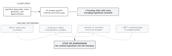
Failure conditions for negative-energy compensation. The diagram is schematic and not to scale; a variational threshold is licensed only for the same smooth pulse family, QEI, worldline, state class, and geometric regime used to derive it.
Domain and failure conditions
Section titled “Domain and failure conditions”See the chapter domain and failure-conditions table. The operator application uses the four-dimensional free massless scalar inertial QEI and smooth compact pulses. It does not prove a universal interest rate, constrain stationary boundary energy, or cover pulse separations beyond the local curved-QEI regime.
Exercise
Section titled “Exercise”Derive the variational lower bound on from the sampled QEI.
Solution
Substitution gives . For ,
The inequality must hold for every admissible , so take the supremum and replace a negative result by the trivial bound .