Stochastic Coarse-Graining and Its Derivation from QFT

Stochastic inflation arises by separating a light scalar into long and short modes with a moving physical scale and then approximating the short-mode crossings as noise. The leading white Gaussian result requires a sharp window, a BD-like short state, weakly varying $H$, slow long dynamics, and a hierarchy between the crossing time and relaxation time.

Required background. de Sitter infrared regimes fixes the object and limits; interacting secular logs fixes the leading-long series; infrared resummation fixes the relaxation scale; and influence functionals fixes the reduced description. Helpful background. Review decoherence claims and open-system EFT.

A moving long–short split

For a window $W_L(y)$ that is one at small $y$, define

$$\phi_L(t,\mathbf x)= \int\frac{d^3k}{(2\pi)^{3/2}} W_L\!\left(\frac{k}{k_c(t)}\right) \left[a_{\mathbf k}u_k(t)e^{i\mathbf k\cdot\mathbf x} +\text{h.c.}\right], \qquad k_c(t)=\epsilon a(t)H.$$

The parameter satisfies $\epsilon\ll1$, but it must remain large enough that gradients and omitted slow terms are ordered relative to the claimed accuracy. Differentiating $W_L$ produces a shell source as modes cross $k_c$. For a Heaviside window, fixed $H$, a massless BD mode, and one spatial point,

$$\frac{d}{dt}\langle\phi_L^2\rangle =\frac{1}{2\pi^2}k_c^2\dot k_c \lvert u_{k_c}\rvert^2 =\frac{H^3}{4\pi^2}.$$

After neglecting long acceleration and gradients, the leading cosmic-time equation is

$$\dot\phi_L(t,\mathbf x) =-\frac{V'(\phi_L)}{3H}+\zeta(t,\mathbf x),$$

with

$$\langle\zeta(t,\mathbf x)\zeta(t',\mathbf x')\rangle =\frac{H^3}{4\pi^2}\delta(t-t') \frac{\sin[k_c(t)r]}{k_c(t)r}, \qquad r=\lvert\mathbf x-\mathbf x'\rvert.$$

Equivalently, at one point $d\phi_L=-V'dt/(3H)+H^{3/2}dW_t/(2\pi)$ with $\mathbb E[dW_t^2]=dt$. This fixes the factor of two in the Fokker–Planck diffusion coefficient $H^3/(8\pi^2)$.

First application: the free leading logarithm

Set $V'=0$ and initialize the long variance at $t_0$. Itô’s rule gives

$$\langle[\phi_L(t)-\phi_L(t_0)]^2\rangle =\frac{H^3}{4\pi^2}(t-t_0) =\frac{H^2}{4\pi^2}\ln\frac{a(t)}{a(t_0)}.$$

This is the leading superhorizon logarithm of the in-in two-point function with the same initial infrared scale. Adding a light potential supplies the slow-roll drift; iterating it reproduces the leading potential-interaction logarithms. Starobinsky’s original construction derives this long-field Fokker–Planck description and its scalar applications Starobinsky 1986, §§2–4, pp. 109–121.

The split is not a tensor-product factorization fixed once and for all: modes continually cross its moving boundary. A sharp window makes crossings instantaneous and hence white in time. A smooth window spreads one crossing over a finite interval, producing colored noise and window-dependent subleading drift. Initial excitations can also change the noise spectrum. These effects must be matched rather than interpreted as new universal forces.

An open-system derivation shows how diagonal long-field probabilities approach the stochastic description under a Born–Markov hierarchy and supplies corrections Burgess et al. 2015, §§3–4, Eqs. (3.23)–(4.18). Squeezing alone does not prove decoherence or classical stochasticity; the reduced density matrix and the tested observables must justify that replacement.

The structure map displays the moving window between renormalized QFT and the Langevin description. Inspect the state and correlation-time assumptions attached to the noise arrow.

For a light spectator in fixed de Sitter, sharp-window crossings give noise strength $H^3/(4\pi^2)$; smooth windows and nonstandard states modify correlations beyond leading order. Schematic; not to scale.

Domain and failure conditions

Use the chapter’s canonical domain table. The derivation assumes a scalar spectator, fixed or slowly varying $H$, a BD-like short state, weak gradients, a specified window, sufficient decoherence for probabilistic observables, and long relaxation compared with the short correlation time. It does not apply automatically to constrained gravity.

Adversarial test. Replace the step window by two smooth windows and vary $\epsilon$ while matching the long equal-time two-point function at one reference scale. The leading $H^3/(4\pi^2)$ growth must agree within the declared gradient and slow-variation error; residual leading dependence that cannot be absorbed into matching signals a failed split. Then choose a window whose correlation time is comparable to the long relaxation time: white-noise evolution must be downgraded to colored memory.

The failure map sends the reduced equation to Langevin/Fokker–Planck dynamics only after normalization is fixed, and to open-system noise when the Markov hierarchy fails.

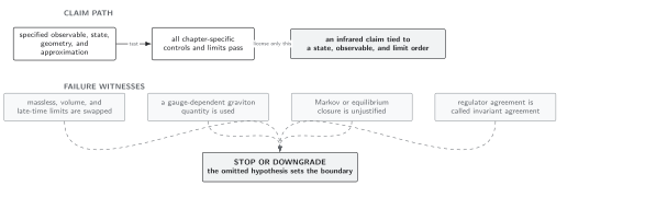
White Gaussian noise is the leading result of a declared scalar hierarchy, not an exact property of every window, state, interaction, or gravitational split. Schematic; not to scale.

References

• Burgess, C. P., R. Holman, G. Tasinato, and M. Williams, “EFT Beyond the Horizon: Stochastic Inflation and How Primordial Quantum Fluctuations Go Classical,” Journal of High Energy Physics 2015(03), 090 (2015), doi:10.1007/JHEP03(2015)090.
• Starobinsky, A. A., “Stochastic de Sitter (Inflationary) Stage in the Early Universe,” in Field Theory, Quantum Gravity and Strings, Lecture Notes in Physics 246, 107–126 (Springer, 1986), doi:10.1007/3-540-16452-9_6.