

Trans-Planckian Initial-State Sensitivity
“Trans-Planckian” sensitivity is not one universal spectrum. A low-energy calculation may parameterize finite-time state preparation by boundary operators suppressed by a physical cutoff, but it cannot determine their Wilson coefficients from semiclassical evolution above that cutoff. A controlled result must connect one operator to a correlator, check the excited-state stress, and show that changing bookkeeping choices does not move the prediction at retained order.
Required background. Initial density matrices and boundary EFT supplies localized state kernels; vacuum choice fixes the reference modes; and gravitational EFT power counting fixes the cutoff. Helpful background. Bunch–Davies and alpha diagnostics distinguish UV-soft excitations from constant alpha mixing.
A dimension-five boundary perturbation
Section titled “A dimension-five boundary perturbation”Let all modes be prepared on one spacelike surface with scale factor . Consider
The integrand is a dimension-four operator on the three-dimensional boundary; written as a four-dimensional insertion with , it is conventionally called dimension five, hence the coefficient .
Here is a physical cutoff, is a real dimensionless renormalized coefficient for this pure-state Robin benchmark, and is physical momentum on . A general mixed closed-time-path kernel would also contain noise data and is not represented by this one real coefficient. Variation shifts the physical Robin kernel by
up to a sign that can be absorbed into . This is a derivative expansion: every retained mode must satisfy
In physical-normal notation the condition is
For the canonical mode , the corresponding conformal-time shift is .
Schalm, Shiu, and van der Schaar derive the boundary-operator organization and its inflationary power-spectrum correction in Schalm, Shiu, and van der Schaar 2004, §§2–4 and §6. Collins and Holman explain the associated initial-surface renormalization in Collins and Holman 2005, §§II–IV.
Robin data produce an explicit Bogoliubov correction
Section titled “Robin data produce an explicit Bogoliubov correction”The simplest transparent benchmark is a subhorizon massless mode, , for which the scale-factor terms in the reference Robin condition are smaller by and
Impose at
The reference mode obeys the condition when . Substitution gives the exact ratio
With , its small- expansion is
The curvature correction is written rather than because this is the boundary-induced difference from the exact reference state: it must vanish together with when the boundary perturbation is removed.
For the late-time massless de Sitter mode in the conventions of the preceding page, the growing field amplitude is proportional to . Therefore
and the first-order boundary signal is
This result is deliberately conditional. On a fixed initial surface, the envelope grows linearly with and the phase is linear in . It is not a universal signal. The coefficient, sign, phase, leading power, and even momentum dependence change with the preparation prescription and operator basis.
The benchmark below displays the signal, its envelope, and the cumulative excitation stress using the same expansion parameter. It is a consistency illustration, not an observational template.
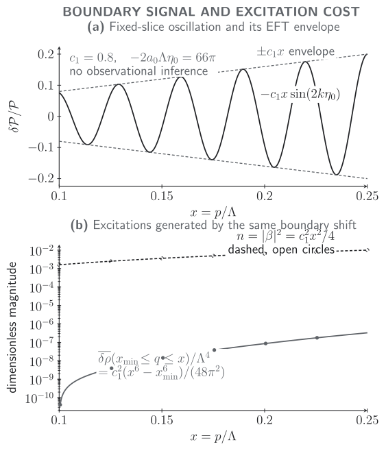
For the stated Robin benchmark on with , the oscillatory power correction has envelope , while and the cumulative time-averaged excitation density scale as and . The band integral vanishes at ; because zero has no logarithmic coordinate, the lower panel begins with the first positive sampled value. Approaching the cutoff increases the apparent signal and simultaneously erodes EFT control. Quantitative benchmark; not an observational fit.
The plotted CSV data and complete machine-readable benchmark state the equations, conventions, frozen inputs, and checks.
Excitation stress and backreaction
Section titled “Excitation stress and backreaction”The particle-like energy formula requires a basis and an averaging statement. In a relativistic adiabatic regime, after local vacuum subtraction and after averaging the rapidly oscillating interference term, the excitation contribution is
It is not the full instantaneous : before averaging, phase-sensitive terms linear in and the required local boundary counterterms can also contribute. The renormalized stress-tensor difference is the correct object when no adiabatic diagonal basis exists.
For the benchmark above, retain the explicit subhorizon band
and use only on that band. The cumulative averaged density on the initial slice is
This exact band integral makes the competing scalings visible: the signal at one momentum is , but filling the controlled band produces an energy cost proportional to . No claim is made about lower momenta, where the deep-subhorizon approximation requires a separate completion. Background control requires at least
For slow-roll predictions, preserving the smaller kinetic source can demand the stronger model-dependent condition . The exact bound must be derived from the background and observable being protected, not selected after seeing the desired signal.
Fixed surface, new-physics hypersurface, and dynamics
Section titled “Fixed surface, new-physics hypersurface, and dynamics”Several proposals called “trans-Planckian initial conditions” are physically inequivalent:
| Preparation | Where data are imposed | Typical momentum dependence | Primary control issue |
|---|---|---|---|
| Fixed-surface boundary EFT | One for all | Amplitude and phase depend on and | Derivative expansion fails first for the shortest retained modes |
| New-physics hypersurface | A different when | Often an envelope with slowly varying phase, given extra adiabatic assumptions | It is not the same state prescription on one Cauchy surface |
| Earlier dynamical preparation | Evolve through a specified UV or heavy-field model | Model-dependent transfer and phases | Adiabaticity, matching, and UV completion must be calculated |
Easther, Kinney, and Peiris show explicitly that fixed-surface boundary EFT and new-physics-hypersurface prescriptions yield radically different spectral dependences in Easther, Kinney, and Peiris 2005, §§II–III. This is a contrary-result check, not a choice between two universal answers.
Likewise, the fact that a late-time EFT mode can be extrapolated to a trans-cutoff physical momentum in the distant past does not by itself prove that the late observable is UV sensitive. Adiabatic evolution can preserve low-energy predictivity even when the earlier description is unavailable; nonadiabatic dependence must be demonstrated Burgess, de Alwis, and Quevedo 2021, §§2–4.
Running, evolution, and moving the initial surface
Section titled “Running, evolution, and moving the initial surface”Two operations are often called “running,” but they are different:
- Changing the subtraction scale is renormalization-group running. The coefficients cancel logarithmic dependence in correlators.
- Moving while representing the same physical state is unitary evolution and matching. The complete density matrix must be evolved to the new surface; when re-expanded in local boundary operators, infinitely many coefficients generally reshuffle.
At finite EFT order, a matched surface move may leave differences of the first omitted order. A leading feature that moves because only the phase was changed—without evolving the state or rematching coefficients—is preparation dependence, not an observable prediction.
Field redefinitions and boundary equations of motion can also move strength among operators. Only the translated correlator is invariant. This is why one coefficient by itself is not an observable and why a visually distinctive oscillation does not relax the power-counting test.
Checks and failure conditions
Section titled “Checks and failure conditions”A controlled result must state the initial surface, physical cutoff, momentum window, operator basis, state completion above the window, subtraction prescription, stress bound, and first omitted order. Reject the result if any of the following occurs:
- some reported mode has of order one;
- violates Bogoliubov normalization or density-matrix positivity;
- the renormalized stress is large enough to change the background being used;
- a leading feature changes under a matched shift of ;
- the result silently replaces a fixed surface by a mode-dependent preparation surface;
- an oscillatory template is interpreted as a measurement of UV microphysics without a specified likelihood and competing low-energy models.
As of 23 August 2026, this page makes no detection claim. The final Planck inflation analysis found no evidence for the parameterized primordial-feature models it tested, including strengthened tests of some oscillatory models using bispectrum data Planck Collaboration 2020, abstract. That result is neither a test of every boundary prescription nor a way to identify the ultraviolet origin of a future feature. A bound on would remain conditional on a chosen state model, momentum window, cosmological parameterization, dataset, likelihood, and nuisance treatment. Those dated observational ingredients belong in a dedicated inference record; the durable result here is the EFT consistency relation among signal, cutoff, and stress.
Common pitfalls
Section titled “Common pitfalls”Writing as an exact identity. It is the first-order term; the quadratic correction is part of the uncertainty when the excitation is not infinitesimal.
Calling the exact stress tensor. It is the diagonal, relativistic, averaged excitation contribution in a declared basis. The full instantaneous renormalized stress can contain interference and local counterterm terms.
Equating subtraction-scale running with time evolution. Changing and moving the initial Cauchy surface solve different consistency problems.
Exercises
Section titled “Exercises”Derive the Bogoliubov ratio produced by the Robin shift and obtain the leading late-time power correction.
Solution
At ,
whereas
Applying the boundary condition to gives
Using yields
At late times the massless de Sitter growing mode is proportional to , so
Integrate the averaged excitation energy over the controlled band to and turn the background inequality into a bound on .
Solution
On the initial slice, change variables from to :
With ,
The conservative background condition becomes
This integrated bound does not replace the mode-by-mode requirement ; both must hold. A slow-roll observable may replace the right-hand energy scale by the smaller .
References
Section titled “References”- Burgess, C. P., S. P. de Alwis, and F. Quevedo, “Cosmological Trans-Planckian Conjectures Are Not Effective,” Journal of Cosmology and Astroparticle Physics 2021, 037 (2021), doi:10.1088/1475-7516/2021/05/037, Open PDF.
- Collins, H., and R. Holman, “Renormalization of Initial Conditions and the Trans-Planckian Problem of Inflation,” Physical Review D 71, 085009 (2005), doi:10.1103/PhysRevD.71.085009.
- Easther, R., W. H. Kinney, and H. Peiris, “Boundary Effective Field Theory and Trans-Planckian Perturbations: Astrophysical Implications,” Journal of Cosmology and Astroparticle Physics 2005, 001 (2005), doi:10.1088/1475-7516/2005/08/001, Open PDF.
- Planck Collaboration, “Planck 2018 Results. X. Constraints on Inflation,” Astronomy & Astrophysics 641, A10 (2020), doi:10.1051/0004-6361/201833887, Open PDF.
- Schalm, K., G. Shiu, and J. P. van der Schaar, “Decoupling in an Expanding Universe: Boundary RG-Flow Affects Initial Conditions for Inflation,” Journal of High Energy Physics 2004, 076 (2004), doi:10.1088/1126-6708/2004/04/076, Open PDF.