Tensor Modes and Primordial Gravitons

Primordial tensor perturbations are the transverse-traceless fluctuations of the spatial metric. In minimal single-field inflation they form two canonically normalized helicities, but their interpretation as gravitons and the normalization of their spectrum depend on the metric, polarization, state, and effective-gravity conventions being kept explicit.

Required background. Gauge-invariant inflationary perturbations separates tensors from constrained sectors; background symmetry breaking supplies the FLRW solution; and gravitational EFT power counting supplies the test for higher-curvature corrections.

Helpful background. Relational gravitational observables clarifies the distinction between a gauge-fixed metric correlator and an operational observable.

Two helicities and their canonical modes

Use

$$h_{ij}=a^2(e^\gamma)_{ij}, \qquad \partial_i\gamma_{ij}=0, \qquad \gamma_{ii}=0.$$

The quadratic Einstein action is

$$S_\gamma^{(2)}=\frac{M_{\rm Pl}^2}{8} \int d\eta\,d^3x\,a^2 \left[\gamma_{ij}'\gamma_{ij}'- \partial_\ell\gamma_{ij}\partial_\ell\gamma_{ij}\right].$$

To make all factors visible, expand

$$\gamma_{ij}(\eta,\mathbf x)=\frac1{\sqrt2} \sum_{\lambda=\pm}\int\frac{d^3k}{(2\pi)^3} e_{ij}^{\lambda}(\hat{\mathbf k})\, \gamma_\lambda(\eta,\mathbf k)e^{i\mathbf k\cdot\mathbf x},$$

with $e_{ij}^{\lambda}e_{ij}^{\lambda' *}=2\delta_{\lambda\lambda'}$. Then $u_\lambda=aM_{\rm Pl}\gamma_\lambda/2$ is canonical and obeys

$$u_{\lambda k}''+\left(k^2-\frac{a''}{a}\right)u_{\lambda k}=0, \qquad u_{\lambda k}u_{\lambda k}^{*\prime}-u_{\lambda k}'u_{\lambda k}^*=i.$$

In slowly varying inflation, the adiabatic state gives the summed dimensionless spectrum

$$\mathcal P_t(k)=\sum_\lambda\frac{k^3}{2\pi^2} \lvert\gamma_{\lambda k}\rvert^2 =\frac{2H_*^2}{\pi^2M_{\rm Pl}^2} \left[1+O(\epsilon)\right].$$

The star denotes evaluation associated with freeze-out, not an assertion that the mode instantly becomes constant at $k=aH$. These conventions and the two-polarization result follow from the tensor sector of Maldacena 2003, §§2 and 3.4, Eqs. (2.25)–(2.28), (3.20)–(3.23).

What the tensor spectrum predicts

At linear order $\gamma_{ij}$ is invariant under scalar gauge transformations, and each helicity behaves like a massless minimally coupled mode with the gravitational normalization above. For a canonical single clock with tensor speed one, combining the scalar result with the tensor result gives $r=16\epsilon$ at leading order. With scalar sound speed $c_s$, the corresponding minimal relation is $r=16\epsilon c_s$ evaluated with care at the two different crossing times.

Parity invariance makes the two helicity spectra equal. A parity-violating interaction can split them, but then the helicity tensors, complex-conjugation rule $e_{ij}^{\lambda *}(\hat{\mathbf k})=e_{ij}^{\lambda}(-\hat{\mathbf k})$, and the definition of a chiral spectrum must be declared. Statistical isotropy fixes the two-point function to be diagonal in momentum and helicity only for an isotropic state. These are empirical assumptions about the background and state, not consequences of transverse tracelessness alone.

The first application is to solve both helicities in constant slow roll, impose their Wronskians, and sum rather than average them. A missing factor of two can arise from the polarization norm, the $1/\sqrt2$ in the expansion, or a per-helicity versus total definition of $\mathcal P_t$; stating all three removes the ambiguity.

The structure map shows the tensor branch running parallel to the scalar constraint reduction.

Two helicities, their polarization normalization, canonical variables, and state together fix the numerical tensor spectrum. Schematic; not to scale.

Modified gravity and observable limits

An EFT can replace $M_{\rm Pl}^2$ by a time-dependent tensor kinetic coefficient, change the tensor speed, or add higher-spatial-derivative dispersion. Such terms are perturbative only while $H/\Lambda$ and the associated dimensionless Wilson coefficients remain small. If an extra pole enters below the claimed cutoff, it must be treated as a new degree of freedom rather than as a finite correction.

The adversarial check repeats the spectrum with the leading higher-curvature or varying-Planck-mass operator included. Verify positivity of the kinetic term, the dispersion relation, the Wronskian, and the late-time map to a relational or detector observable. A coordinate metric two-point function alone does not establish an observable graviton background.

An additional normalization check follows from the flat limit. For $a$ constant, each canonical $u_\lambda$ must reduce to $e^{-ik\eta}/\sqrt{2k}$ and the equal-time commutator must have the standard delta function. Taking the de Sitter limit afterward must reproduce the total factor of two in $\mathcal P_t$. This two-step check catches polarization conventions that accidentally give the correct tilt but the wrong amplitude.

See the chapter’s domain and failure conditions. The validity map separates normalization errors from a genuine failure of the Einstein two-derivative approximation.

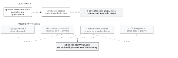
The minimal tensor formula applies only with two healthy helicities, controlled higher-derivative corrections, a normalized state, and a declared observable interpretation. Schematic; not to scale.

References

• Maldacena, J., “Non-Gaussian Features of Primordial Fluctuations in Single Field Inflationary Models,” Journal of High Energy Physics 05, 013 (2003), doi:10.1088/1126-6708/2003/05/013.