Seeley–DeWitt Coefficients and Curvature Invariants

Seeley–DeWitt coefficients are local invariants generated by a transport recursion for a specified Laplace-type operator. Their numerical entries have meaning only together with the Riemann sign, operator endomorphism, bundle connection, coefficient-index convention, boundary assumptions, and invariant basis.

Required background. Heat Kernels and the Schwinger–DeWitt Expansion defines the asymptotic series, and Levi–Civita Connections, Geodesics, and Riemann Curvature supplies the bitensors and curvature identities.

Helpful background. Curvature Counterterms and Composite-Operator Mixing explains why the coefficients enter renormalization; Integration by Parts and Equation-of-Motion Redundancy explains basis reduction.

Transport recursion along the geodesic

For

$$\mathcal D=-\bigl(\nabla_E^2+\mathcal E\bigr),$$

write the off-diagonal kernel as

$$K(s;x,x')\sim\frac{\Delta^{1/2}}{(4\pi s)^{d/2}} e^{-\sigma/(2s)}\sum_{n=0}^{\infty}a_n(x,x')s^n.$$

With the Van Vleck factor displayed, $a_0(x,x')$ is parallel transport in the bundle. The higher coefficients solve

$$\left(\sigma^{;\mu}\nabla_\mu+n\right)a_n =\Delta^{-1/2} \left(\nabla_E^2+\mathcal E\right) \left(\Delta^{1/2}a_{n-1}\right).$$

The left side transports along the unique geodesic; coincidence limits follow by differentiating the recursion and using Synge’s rule. This constructive form is the reason each $[a_n]$ is a polynomial of total mass dimension $2n$. Manifestly covariant algorithms for the coincidence limits and their derivatives are developed in Avramidi 1999, §§ 2–4.

For a general bundle, define

$$\Omega_{\mu\nu}=[\nabla_\mu,\nabla_\nu]_{\rm bundle}.$$

The first coincidence limits in this chapter’s $s^n$ notation are

$$[a_0]=\mathbf1, \qquad [a_1]=\mathcal E+\frac16R_E\mathbf1,$$

and

$$\begin{aligned} [a_2]=\frac1{360}\bigl(&60\nabla_E^2\mathcal E +60R_E\mathcal E+180\mathcal E^2+30\Omega_{\mu\nu}\Omega^{\mu\nu}\\ &+12\nabla_E^2R_E+5R_E^2 -2R_{\mu\nu}R^{\mu\nu} +2R_{\mu\nu\rho\sigma}R^{\mu\nu\rho\sigma}\bigr). \end{aligned}$$

These are Vassilevich’s $a_0,a_2,a_4$ because that source indexes by derivative dimension Vassilevich 2003, Eqs. (4.26)–(4.28).

The off-diagonal recursion supplies more than the integrated divergence. Derivatives of $a_n(x,x')$ control point-split composite operators and stress-tensor variations, so taking coincidence too early can discard required tensor data. A robust calculation verifies the exchange symmetry appropriate to the bundle adjoint, then traces, integrates, and reduces the invariant basis in that order. On a constant-curvature test space, all derivative terms vanish and the remaining polynomial must scale as $R_E^n$; this catches both index shifts and missing connection-curvature terms.

First application: arbitrary scalar curvature coupling

For the Euclidean scalar crosswalk

$$\mathcal L_E=-\nabla_E^2+m^2-\xi R_E,$$

factor out $m^2$ and identify $\mathcal E=\xi R_E$. Because a scalar has $\Omega_{\mu\nu}=0$,

$$[a_1]=\left(\xi+\frac16\right)R_E,$$ $$\begin{aligned} [a_2]={}&\frac1{180} (R_{\mu\nu\rho\sigma}^2-R_{\mu\nu}^2) +\frac12\left(\xi+\frac16\right)^2R_E^2\\ &+\left(\frac1{30}+\frac\xi6\right)\nabla_E^2R_E. \end{aligned}$$

The checks are independent and strong:

• dimensions are $0,2,4$;
• $[a_1]$ vanishes at $\xi=-1/6$;
• flat space leaves only $[a_0]$ after the mass factor is separated;
• on a closed manifold the integrated Laplacian vanishes, but the local coefficient retains it;
• replacing $\xi$ by $-\xi_c$ yields the familiar $(1/6-\xi_c)R_E$.

In four dimensions the quadratic-curvature part can instead be written

$$[a_2]=\frac1{120}C_{\mu\nu\rho\sigma}^2 -\frac1{360}E_4 +\frac12\left(\xi+\frac16\right)^2R_E^2 +\left(\frac1{30}+\frac\xi6\right)\nabla_E^2R_E,$$

where $E_4=R_{\mu\nu\rho\sigma}^2-4R_{\mu\nu}^2+R_E^2$. This basis change uses only the four-dimensional algebraic identities; it is not valid unchanged in arbitrary $d$ during dimensional continuation.

Convention and basis adversary

Take a source with the opposite Riemann-tensor sign. A reliable translation starts from its operator $\mathcal D$, recomputes $\mathcal E$ and $\Omega_{\mu\nu}$ in the site convention, and only then uses the universal polynomial. Flipping printed $R$ while leaving $\mathcal E$, $\xi$, the commutator curvature, or the Laplacian term untouched is inconsistent. Curvature squares can conceal the mistake because they are even under a simultaneous sign flip, whereas $[a_1]$ and $\nabla^2R$ expose it.

Integration by parts and Gauss–Bonnet reduction may move coefficients among $R_{\mu\nu\rho\sigma}^2$, $R_{\mu\nu}^2$, $R^2$, and $\nabla^2R$. The integrated divergence on the same domain must remain unchanged. If it does not, the comparison has mixed dimensions, discarded a boundary term, or changed conventions incompletely.

The structure map shows the coefficients between the heat kernel and every local counterterm. Inspect the distinction between a local coefficient and the later basis chosen for matching.

The operator determines the coefficient polynomial; tracing, integrating, and choosing an invariant basis are subsequent operations that can remove or rearrange terms. Schematic; not to scale.

Domain and failure conditions

The formulas assume a smooth Laplace-type operator without a boundary. Nonminimal operators, distributional potentials, mixed boundary conditions, and conical strata have additional structures. The table at Domain and failure conditions records which outputs survive.

The failure map’s convention branch is caught by three fixtures: the conformal zero of $[a_1]$, a constant-curvature background, and equality of the integrated divergence before and after basis reduction.

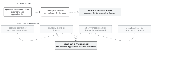
Coefficient tables are comparable only after operator, Riemann sign, bundle curvature, dimension, total derivatives, and basis have all been translated. Schematic; not to scale.

Handoffs

Heat Kernels with Boundaries and Conical Singularities adds localized coefficients. Renormalization of Gravitational Couplings by Matter Loops converts the closed-manifold coefficients into counterterms and scale dependence.

References

• Avramidi, Ivan G. “Covariant Techniques for Computation of the Heat Kernel.” Reviews in Mathematical Physics 11 (1999): 947–980. DOI. Open PDF.
• Vassilevich, Dmitri V. “Heat Kernel Expansion: User’s Manual.” Physics Reports 388 (2003): 279–360. DOI. Open PDF.