False-Vacuum Decay with Gravity: Regime and Observable Contract

A gravitational decay calculation becomes definite only after the metastable state, spacetime and boundary data, observable, clock, contour, and approximation hierarchy have been chosen. A local rate per proper four-volume, the survival probability of a region, and the physical false-vacuum volume on a foliation are related only through a geometric integral. They are not interchangeable probability statements.

Required background. Fixed-background, semiclassical, EFT, and quantum-gravity regimes fixes which variables fluctuate; the semiclassical Einstein equation fixes mean backreaction; and vacuum-decay validity and gravity handoffs supplies the flat-space stopping rules.

Helpful background. Metastability and spinodals separates nucleation from barrier disappearance, while imaginary parts and vacuum instability distinguishes an effective-action signal from a prepared-state probability.

Three observables before one method

Let $\rho_F$ be a prepared metastable state for a scalar potential with false minimum $\phi_F$, lower minimum $\phi_T$, and barrier scale $M_b$. The following objects answer different questions.

Local dilute-instanton rate. In a slowly varying region, define a scalar rate density $\Gamma_4(x)$ by

$$dN_{\mathrm{nuc}} =\Gamma_4(x)\,d^4x\,\sqrt{-g}.$$

This definition is invariant. A nearly constant $\Gamma_4$ is meaningful only when the state and geometry change slowly across a critical bubble and on the mean waiting time.

Regional survival. For a false-sector effect or projector $\Pi_F(\Sigma_t)$ on a chosen slice,

$$P_F(t) =\operatorname{Tr}\!\left[ \Pi_F(\Sigma_t)\, U(t,t_0)\rho_FU(t,t_0)^\dagger \right].$$

This depends on the initial state, slice, region, and definition of “false.” In a Poisson window it may equal an exponential of an integrated local rate, but exact unitary evolution need not be exponential at early or late times.

Cosmological false-vacuum fraction. Given nucleation and wall propagation, $p_F(t)$ is the probability that a comoving point remains false, while

$$V_F^{\mathrm{phys}}(t)\propto a(t)^3p_F(t)$$

tracks expected physical volume in a specified slicing. A decreasing fraction can coexist with a growing physical volume.

The structure map makes method selection downstream of this choice. Euclidean, closed-time-path, and stochastic calculations can agree on an exponent in an overlap regime while computing different primary objects.

Observable-first regime selection. The diagram is schematic and not to scale; agreement between methods is meaningful only after their state, region, clock, and normalization have been matched.

Weak-gravity scalar classification

For a critical bubble of radius $R_b$ and wall thickness $\ell_w$, a useful controlled hierarchy is

$$B\gg1, \qquad \ell_w\ll R_b, \qquad R_b\Lambda_{\mathrm{EFT}}\gg1, \qquad R_b^2\lvert R_{\mu\nu\rho\sigma}\rvert\ll1$$

for a thin-wall, weak-curvature saddle. Weak gravitational coupling can also be monitored by $\kappa(\Delta\phi)^2\ll1$, with $\kappa=8\pi G$, but this alone does not guarantee small gravitational effects when vacuum energies make $H R_b$ order unity.

Classify the same potential in three ways.

1. Euclidean question: fix the induced boundary geometry or use a regular compact manifold; find all relevant saddles; compute the matched action difference $B$; identify the integration contour and physical negative mode; and estimate determinants. The strongest output before the last two steps is a saddle exponent.
2. Real-time question: fix $\rho_F$, the false-sector observable, and an initial Cauchy surface; evolve on a closed time path; and extract $-\partial_t\log P_F$ only over a demonstrably exponential interval. Batini, Chatrchyan, and Berges find time-dependent rates at next-to-leading order in a large-$N$ two-particle-irreducible benchmark, illustrating why the initial-value problem contains more information than a constant exponent (Batini, Chatrchyan, and Berges 2024, §§ II and V–VI).
3. Cosmological question: supply $\Gamma(t)$ or $\Gamma(T)$ with covariance, solve $H(t)$ and $T(t)$, propagate walls, and compute nucleation, percolation, and completion separately. This calculation consumes the microscopic rate rather than redefining it.

A common EFT error estimate should include loop suppression, derivative and curvature corrections, thin-wall corrections when used, and sensitivity to finite gravitational couplings. If any correction is comparable with $B$ at the requested precision, exponential sensitivity magnifies it:

$$\frac{\delta\Gamma_4}{\Gamma_4} \simeq \frac{\delta A}{A}-\delta B.$$

Thus a “percent-level rate” requires substantially tighter control of the action than a percent-level field profile.

Rate-to-survival adversarial test

Suppose $\Gamma_4$ is constant in a de Sitter flat slicing. The probability that a chosen comoving worldline has not been reached by a bubble is, in a dilute independent-nucleation model,

$$P_F(t)=e^{-I(t)},$$

with

$$I(t) =\frac{4\pi}{3} \int_{t_0}^{t}dt'\, \Gamma_4\,a(t')^3 \left[ \int_{t'}^{t}\frac{v_w(t'')}{a(t'')}\,dt'' \right]^3.$$

The invariant rate enters, but $P_F(t)$ depends on the slicing through $a(t)$ and the chosen equal-time bubble volume, and on the wall speed and initial time. Relabelling time by $N=Ht$ is harmless only after transforming the probability density and integration measure. Treating $\Gamma_4 t$ as the exponent drops three powers of the causal radius and is dimensionally wrong.

The strongest invariant statement that survives a foliation change is the local proper-volume rate together with a covariant description of the affected spacetime region. A survival curve survives only after its region and foliation are carried through the transformation.

The failure map marks the first unsupported promotion—from saddle to rate, rate to survival, or survival to global volume.

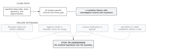
Failure tests for the decay contract. The diagram is schematic and not to scale; each promotion requires additional state, geometric, contour, or measure data.

Domain and failure conditions

See the chapter domain and failure-conditions table. The weak-gravity classification assumes a metastable prepared state, a scalar EFT with a resolved wall, a dilute saddle expansion, and curvature below the cutoff. It does not define a probability for the entire spacetime, cover spinodal evolution after the barrier disappears, or supply a global measure.

Exercise

Show that $\Gamma_4t$ cannot be the exponent of a four-dimensional survival probability for a constant proper-volume rate.

Solution

In four spacetime dimensions, $\Gamma_4$ has mass dimension four and $t$ has dimension minus one, so $\Gamma_4t$ has dimension three. A dimensionless exponent requires an integrated four-volume:

$$I=\int_{\mathcal R}d^4x\,\sqrt{-g}\,\Gamma_4.$$

The region $\mathcal R$ is fixed by the survival question—for example, the past domain from which a bubble wall can reach the chosen event.

References

• Batini, L., A. Chatrchyan, and J. Berges. “Real-Time Dynamics of False Vacuum Decay.” Physical Review D 109 (2024): 023502. DOI. Open PDF.
• Coleman, S. “The Fate of the False Vacuum. I. Semiclassical Theory.” Physical Review D 15 (1977): 2929–2936; erratum 16 (1977): 1248. DOI.
• Coleman, S., and F. De Luccia. “Gravitational Effects on and of Vacuum Decay.” Physical Review D 21 (1980): 3305–3315. DOI.