

Reconstruction from Symmetry, Singularities, and Cuts
Symmetry, factorization, cuts, and locality can reconstruct the nonlocal part of many tree-level cosmological coefficients. They determine a unique answer only when the allowed homogeneous contact space is empty or separately fixed. A complete result therefore returns a solution class, a basis for its local freedom, and the extra data needed to select one representative.
Required background. Ward identities, factorization singularities, cosmological cuts, and locality and field-redefinition equivalence provide the four inputs.
Helpful background. Subtracted dispersion relations organize analytic freedom, and the amplitude bootstrap supplies the flat-space analogue.
Reconstruction as an inhomogeneous problem
Section titled “Reconstruction as an inhomogeneous problem”Let denote the relevant Ward or differential operator and let channel data supply an inhomogeneous source :
If is one solution, the general answer is
Factorization and cuts constrain the singular part of . Locality restricts to a finite contact basis only after an EFT derivative bound, field-redefinition quotient, and late-boundary prescription are imposed:
The coefficients may be fixed by a total-energy contact amplitude, a soft theorem, matching to a Lagrangian or observation, or an ultraviolet assumption. Without that input they are physical Wilson data or scheme-dependent boundary data, not reconstruction errors.
Four-point exchange application
Section titled “Four-point exchange application”For identical scalars with a specified -channel internal particle, begin with an ansatz whose only nonanalytic channel surfaces are
plus the known massive branch cuts. Match the and residues or discontinuities to products of normalized three-point data. Impose the state-specific cut identity and remove spurious poles. In the conformal rational benchmark this produces
Crossing symmetry for identical external fields then gives
This expression has the required channel residues and cutting data. It is not the most general local tree coefficient.
To enumerate the surviving ambiguity, declare a parity-even, generally covariant scalar EFT in exact de Sitter and quotient integrations by parts and the free equation of motion. Through four bulk derivatives, a representative four-field contact basis contains
with curvature-dressed degenerate with the first operator on exact de Sitter and two-derivative four-field terms redundant modulo lower-derivative terms and field redefinitions. Each operator produces a contact seed . Independent late-boundary counterterms must be listed separately. If time diffeomorphisms are broken, fields are distinguishable, or a higher derivative order is allowed, the basis enlarges.
The reconstructed class is thus
Channel residues and cuts do not determine , , or finite boundary coefficients. A supplied full flat-space total-energy amplitude can fix the corresponding bulk contact combination, but not a pure wavefunction phase at the late boundary.
Jazayeri, Pajer, and Stefanyszyn derive partial-energy recursion and manifest-locality tests that fix exchange correlators up to boundary and contact data (Jazayeri, Pajer, and Stefanyszyn 2021, §§ 3–5).
A reproducible reconstruction workflow
Section titled “A reproducible reconstruction workflow”- Define the object. Record wavefunction or correlator, field basis, state, branches, and normalization.
- Choose an ansatz space. State permutation symmetry, tensor basis, derivative bound, and allowed analytic growth.
- Match physical singularities. Fix total- and partial-energy residues or discontinuities on declared sheets.
- Impose cuts. Use the correct density-matrix and branch rule.
- Cancel spurious structure. Enforce Ward identities, locality tests, and soft constraints.
- Compute the null space. Construct every homogeneous contact and subtraction solution.
- Validate independently. Compare a direct bulk integral or differential equation and test all limits.
Numerical sampling can test identities at generic momenta, but it cannot prove that an omitted rational or logarithmic homogeneous solution is absent. The analytic null-space calculation is essential.
Identical-nonlocal-data adversarial test
Section titled “Identical-nonlocal-data adversarial test”Construct
They have identical exchange residues and internal cuts, pass the same exchange factorization tests, and differ by an allowed local interaction. Feed both to the reconstruction algorithm. If it silently returns one coefficient, it has inserted an unreported boundary condition or prior.
The strongest valid output is either the pair’s equivalence class modulo the chosen contact quotient or a unique member after an independent datum fixes . “Minimal” contact content is a convention unless a power counting or ultraviolet principle defines it.
The structure map shows constraints converging on the nonlocal solution before a separate local basis is added. Inspect where uniqueness requires additional input.

Conditional reconstruction of a cosmological boundary coefficient. The diagram is schematic and not to scale; uniqueness is a conclusion only after the homogeneous local null space has been computed.
The failure map tests hidden priors. Inspect the stop triggered by two functions with identical nonlocal data and different allowed contacts.
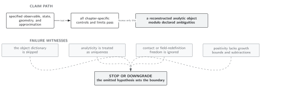
Failure conditions for reconstruction from cosmological analytic data. The diagram is schematic and not to scale; selecting one contact completion without extra input is not reconstruction from singularities.
These limits refine the chapter’s domain and failure conditions. Their stability beyond standard-state tree level is assessed in loops, initial states, and validity.
Exercise
Section titled “Exercise”Let have a known simple pole and satisfy at large . Find the most general addition with no pole and the same growth bound.
Solution
The difference between any two solutions is entire and grows at most linearly. By the polynomial form of Liouville’s theorem, it is
Therefore
The residue fixes the nonlocal pole, while two subtraction or contact constants remain.