In-In Effective Actions and Causal Mean Backreaction

Real-time backreaction is an initial-value problem for expectation values. The closed-time-path, or in-in, effective action doubles the metric history, inserts the initial density matrix at a finite initial surface, and yields a real retarded equation when the two histories are identified after variation. An in-out effective action instead controls transition amplitudes and can give complex, acausal-looking equations if used for evolution.

Required background. One-loop effective actions supplies the matter determinant; closed-time-path practice supplies doubled sources; and influence functionals supplies the reduced mean-field construction.

Helpful background. Noise, dissipation, and fluctuation relations distinguishes the imaginary influence action from mean response; initial density matrices fixes contour boundary data; and in-out versus in-in observables supplies the operational distinction.

Doubled histories and the physical variation

For an initial matter density matrix $\rho_i$ at $t_i$, define

$$Z[g_+,g_-] =\operatorname{Tr}\!\left( U_{g_+}(t_f,t_i)\rho_i U_{g_-}(t_f,t_i)^\dagger \right).$$

The two histories agree at the return surface $t_f$ but are varied independently. The closed-time-path effective action has the form

$$\Gamma_{\rm CTP}[g_+,g_-] =S_g[g_+]-S_g[g_-] +\Gamma_{\rm m,CTP}[g_+,g_-;\rho_i].$$

The mean equation is

$$\left. \frac{\delta\Gamma_{\rm CTP}} {\delta g_+^{\mu\nu}(x)} \right|_{g_+=g_-=g}=0.$$

Unitarity gives $\Gamma_{\rm CTP}[g,g]=0$, while branch exchange supplies the reality relation that makes the physical equation real. Because the contour begins at $t_i$, variation at $x$ depends only on state data and metric history in $J^-(x)$, together with contact terms at the initial surface. Jordan’s construction gives the expectation-value field equation directly and explains why the in-out boundary condition is the wrong one for this task (Jordan 1986, §§ II–IV).

Introduce average and difference variables,

$$g_c=\frac{g_++g_-}{2}, \qquad g_\Delta=g_+-g_-.$$

To keep the metric factors visible, write

$$k_\pm^{\mu\nu}=\delta g_\pm^{\mu\nu}, \qquad k_c=\frac{k_++k_-}{2}, \qquad k_\Delta=k_+-k_-.$$

The matter source is $j^{\mu\nu}=k^{\mu\nu}/2$ because $\delta S_{\rm m}=\frac12\int d\mu\,T_{\mu\nu}\delta g^{\mu\nu}$. With

$$\mathcal R^{\rm R}_{\mu\nu\rho\sigma}(x,y) =+i\theta(x\succ y) \left\langle [\hat T_{\mu\nu}(x),\hat T_{\rho\sigma}(y)] \right\rangle +\mathcal R^{\rm contact}_{\mu\nu\rho\sigma}(x,y),$$

the matter part of the closed-time-path action has the quadratic expansion

$$\begin{aligned} \Gamma_{\rm m,CTP} =\Gamma_{\rm m,CTP}^{(0)} &+\frac12\int d\mu_x\, k_\Delta^{\mu\nu}(x) \langle T_{\mu\nu}(x)\rangle \\ &+\frac14\int d\mu_xd\mu_y\, k_\Delta^{\mu\nu}(x) \mathcal R^{\rm R}_{\mu\nu\rho\sigma}(x,y) k_c^{\rho\sigma}(y) \\ &+\frac{i}{8}\int d\mu_xd\mu_y\, k_\Delta^{\mu\nu}(x) N_{\mu\nu\rho\sigma}(x,y) k_\Delta^{\rho\sigma}(y) +O(k^3). \end{aligned}$$

Here $N_{\mu\nu\rho\sigma}=\frac12\langle\{t_{\mu\nu},t_{\rho\sigma}\}\rangle$ with $t=T-\langle T\rangle$. Consequently the nonlocal stress variation is

$$\delta\langle T_{\mu\nu}(x)\rangle =\frac12\int d\mu_y\, \mathcal R^{\rm R}_{\mu\nu\rho\sigma}(x,y) k^{\rho\sigma}(y).$$

This $+i$ commutator sign follows the site’s plus-source convention. If instead one perturbs the covariant metric, $h_{\mu\nu}=\delta g_{\mu\nu}$, then $k^{\mu\nu}=-h^{\mu\nu}$ to first order and the response coefficient multiplying $h$ is $-\mathcal R^{\rm R}/2$. This crosswalk explains the common $-i/2$ retarded stress kernel in covariant-metric equations without changing the spectral convention. The mean equation comes from the term linear in $k_\Delta$ and contains $\mathcal R^{\rm R}$. The positive noise kernel $N$ enters stress fluctuations and stochastic metric variance, not the deterministic mean equation. Discarding it is a limitation of the mean description, not proof that it is zero.

The structure map’s central arrow is precisely this retarded variation. Its constraint checkpoint also requires the contact terms implied by diffeomorphism Ward identities.

Closed-time-path route to causal mean backreaction. The diagram is schematic and not to scale; branch identification occurs only after variation, and the displayed mean response omits the separate fluctuation sector.

The failure map’s first witness is literal: a Feynman kernel is time ordered, not retarded, and generally has support on both sides of the observation time.

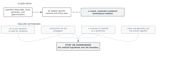
Causality test for a backreaction equation. This schematic, not-to-scale map stops an evolution claim when contour boundary conditions, initial-state terms, reality, or retarded support are missing.

Application: a homogeneous metric memory term

Let $q(t)$ be a homogeneous metric degree of freedom, such as a small perturbation of $\log a(t)$. Define its conjugate operator by the plus-source coupling $S_{\rm int}=+\int dt\,q(t)\hat O(t)$. Expanding the CTP action gives

$$\mathcal D_0q(t) +\int_{t_i}^{t}\!ds\, \Pi_{\rm R}(t,s)q(s) =J_{\rm state}(t),$$

where

$$\Pi_{\rm R}(t,s) =+i\theta(t-s) \langle[\hat O(t),\hat O(s)]\rangle_{\rho_i} +\Pi_{\rm local}(t,s).$$

$\mathcal D_0$ contains the classical and renormalized local curvature terms. $J_{\rm state}$ includes the one-point stress and any initial-surface correlations. The upper integration limit makes causality explicit. For a stationary state, $\Pi_{\rm R}(t,s)=\Pi_{\rm R}(t-s)$, but for a prepared cosmological state it generally remembers both times separately.

To reproduce the calculation, specify $t_i$, $\rho_i$, the preparation or switching prescription, the operator normalization, local counterterms, and the numerical memory cutoff. Verify:

$$\Pi_{\rm R}(t,s)=0\quad\text{for }s>t, \qquad \nabla^\mu\delta\langle T_{\mu\nu}\rangle +(\delta\nabla^\mu)\langle T_{\mu\nu}\rangle=0$$

after contact terms, the state variation, and the background equations are included. The separated-point commutator need not be transverse by itself. Varying the memory cutoff tests tail error; varying $t_i$ without transporting the state tests a different physical preparation, not a numerical uncertainty.

Adversarial test: substitute the Feynman kernel

The in-out quadratic action contains

$$\Pi_{\rm F}(t,s) =-i\langle\mathcal T\hat O(t)\hat O(s)\rangle.$$

It is nonzero for $s>t$ and may have an imaginary part describing production in a transition amplitude. Replacing $\Pi_{\rm R}$ by $\Pi_{\rm F}$ therefore makes $q(t)$ depend on future values and can make a real initial datum evolve through a complex equation. Taking only its real part does not restore the missing initial-state and commutator structure.

The strongest surviving interpretation is an in-out stationary condition for a matrix element. Restoring doubled histories, the initial density matrix, and the retarded kernel licenses causal mean evolution. Fluctuations still require the $N$ kernel and belong to a different observable.

Domain and failure conditions

See the chapter domain and failure-conditions table. The CTP equation is causal within the chosen globally hyperbolic region and initial-state prescription. It requires renormalized local contact terms, a state with admissible short-distance structure, and a consistent truncation of the loop expansion. It does not convert an open-system influence action into a deterministic account of stress noise.

Exercise

Show that the physical CTP equation is insensitive to the arbitrary return time $t_f$ when $t_f$ lies to the future of the observation.

Solution

On the common segment after the latest insertion, forward and backward evolution cancel:

$$U(t_f,t)^\dagger U(t_f,t)=1.$$

Moving $t_f$ farther into the future inserts another unitary factor and its inverse. The retarded kernel therefore depends on the initial surface and causal past of $t$, not on the return time.

Handoff

Constraints and the Bianchi identity show how diffeomorphism Ward identities make this retarded source compatible with gravitational constraints.

References

• Calzetta, Esteban, and Bei-Lok Hu. “Closed-Time-Path Functional Formalism in Curved Spacetime: Application to Cosmological Back-Reaction Problems.” Physical Review D 35 (1987): 495–509. doi:10.1103/PhysRevD.35.495.
• Jordan, R. D. “Effective Field Equations for Expectation Values.” Physical Review D 33 (1986): 444–454. doi:10.1103/PhysRevD.33.444.
• Schwinger, Julian. “Brownian Motion of a Quantum Oscillator.” Journal of Mathematical Physics 2 (1961): 407–432. doi:10.1063/1.1703727.