Linear Response and Semiclassical Stability

Linear response asks whether a self-consistent mean solution remains close to itself under small, admissible perturbations of both geometry and state. The relevant equation contains the retarded stress response, not an in-out polarization tensor. A physical instability must survive the constraints and gauge quotient, lie within the effective theory’s frequency range, and grow relative to the background on the interval of interest. This criterion concerns the mean response; stress fluctuations require additional correlation functions.

Required background. The semiclassical Einstein equation defines the background; in-in effective actions and causal backreaction supplies the retarded kernel; and retarded, advanced, and spectral correlators fixes causal and Fourier conventions.

Helpful background. Order reduction and runaway prescriptions treats cutoff branches, while EFT truncation errors and breakdown diagnostics bounds the trusted frequency domain.

Retarded variation of a self-consistent solution

Let $(\bar g,\bar\omega)$ solve the renormalized mean equation, and perturb it by the covariant metric $h_{\mu\nu}=\delta g_{\mu\nu}$ and compatible state data $\delta\omega$. To first order, $\delta g^{\mu\nu}=-h^{\mu\nu}$. With

$$T_{\mu\nu}=\frac{2}{\sqrt{-g}}\frac{\delta S_{\mathrm m}}{\delta g^{\mu\nu}},$$

the linearized equation has the form

$$\delta\mathcal L_{\mu\nu}[h](x) =8\pi G\left[ \delta T_{\mu\nu}^{\mathrm{state}}(x) +\int dV_y\, \Pi^{\mathrm{ret}}_{\mu\nu}{}^{\rho\sigma}(x,y) h_{\rho\sigma}(y)\right].$$

Here $\delta\mathcal L$ includes the linearized Einstein, cosmological, and fixed finite curvature-counterterm tensors. A convenient definition of the nonlocal part is

$$\Pi^{\mathrm{ret}}_{\mu\nu\rho\sigma}(x,y) =-\frac{i}{2}\,\theta(x\succ y) \left\langle \left[T_{\mu\nu}(x),T_{\rho\sigma}(y)\right] \right\rangle +\Pi^{\mathrm{contact}}_{\mu\nu\rho\sigma}(x,y),$$

where the factor $1/2$ comes from $\delta S_{\rm m}=\frac12\int dV\,T_{\rho\sigma}\delta g^{\rho\sigma}$, and the minus sign comes from varying $g_{\rho\sigma}$ rather than $g^{\rho\sigma}$. For an inverse-metric perturbation $k^{\rho\sigma}=\delta g^{\rho\sigma}$, the nonlocal coefficient is instead $+i\theta\langle[T,T]\rangle/2$; the contact terms transform with the same change of variable. The contact term above is fixed by metric variation of the composite operator and the renormalization prescription. The notation $x\succ y$ means that $x$ is causally to the future of $y$. With this support, compactly supported perturbations of the metric cannot change the mean stress outside their causal future.

Diffeomorphism invariance gives a linearized Ward identity. Schematically,

$$\bar\nabla^\mu \left[ \delta T_{\mu\nu}^{\mathrm{state}} +\Pi^{\mathrm{ret}}_{\mu\nu}[h] \right] +(\delta\nabla^\mu)\, \langle T_{\mu\nu}\rangle_{\bar\omega}=0.$$

The local contact terms are essential to this equality. Dropping them can make a transverse kernel appear nontransverse and can spoil constraint propagation.

The structure map emphasizes that stability is tested after causal response and constraints have been assembled, and before a perturbation is accepted as a nearby self-consistent geometry.

Linear-response stability of a semiclassical mean solution. The map is schematic and not to scale; gauge and constraint directions are removed, and cutoff-scale roots are classified separately from low-energy instabilities.

Poles, initial data, and a usable stability criterion

On a stationary homogeneous background, decompose a gauge-invariant physical channel into spatial momentum $\mathbf k$ and use

$$h(t,\mathbf k)=\int_{\mathcal C}\frac{d\omega}{2\pi}\, e^{-i\omega t}\,\widetilde h(\omega,\mathbf k).$$

The retarded inverse response is

$$\mathcal D_{\mathrm R}(\omega,\mathbf k) =\mathcal D_{\mathrm{loc}}(\omega,\mathbf k) -8\pi G\,\Pi_{\mathrm R}(\omega,\mathbf k).$$

Zeros of $\mathcal D_{\mathrm R}$ determine homogeneous modes, while branch cuts encode multiparticle or continuum response. With the stated $e^{-i\omega t}$ convention, a pole with $\operatorname{Im}\omega>0$ grows, one with $\operatorname{Im}\omega<0$ decays, and a real pole requires its residue and boundary prescription to be examined. A pole alone is not yet physical: it may lie in a gauge sector, violate a constraint, or occur at $\lvert\omega\rvert\gtrsim\Lambda_{\mathrm{EFT}}$.

A practical criterion is therefore:

Every finite, gauge-invariant perturbation generated by admissible compact initial data remains bounded—up to declared physical secular effects—throughout the EFT-controlled interval after constraints and state perturbations are imposed.

Anderson, Molina-París, and Mottola formulate linear response as a necessary validity test and explicitly separate gauge-invariant perturbations from Planck-scale solutions (Anderson, Molina-París, and Mottola 2003, §§ II and V). It is not a sufficient test of all quantum metric fluctuations: the symmetrized stress two-point function, or noise kernel, is absent from the mean equation.

Stationary homogeneous application

For a spatially homogeneous physical perturbation, construct $\mathcal D_{\mathrm R}(\omega,\mathbf0)$ in four steps:

1. vary the local gravitational tensors and the renormalized mean stress in one finite scheme;
2. compute the in-in stress commutator in the chosen background state;
3. impose the linearized Hamiltonian and momentum constraints, then project out pure diffeomorphisms; and
4. locate poles and cuts only inside a stated domain $\lvert\omega\rvert<\eta\Lambda_{\mathrm{EFT}}$ with $\eta<1$.

Changing a finite $R^2$ coupling moves a local polynomial between $\mathcal D_{\mathrm{loc}}$ and the contact part of $\Pi_{\mathrm R}$. If the coupling is translated consistently, the low-energy zeros do not change. Varying only the kernel is not a scheme comparison.

The adversarial test adds two trial perturbations. The first is $h_{\mu\nu}=2\bar\nabla_{(\mu}\xi_{\nu)}$ with compactly supported $\xi$: every gauge-invariant response must vanish even if a gauge-fixed component grows. The second has frequency of order the curvature-squared scale: it may be a true root of the truncated equation, but it is rejected unless the ultraviolet completion or an untruncated response controls it.

As of August 2026, rigorous stability results remain model- and hypothesis-specific. Meda and Pinamonti prove polynomial decay in a scalar toy model for a massive quantum field under sufficient parameter conditions; they do not establish stability for arbitrary semiclassical Einstein backgrounds (Meda and Pinamonti 2023, abstract and Theorem 4.4). Thus the pole workflow is a controlled diagnostic, not a general stability theorem.

The failure map organizes the rejections. A growing component becomes evidence for a physical mean instability only after it survives every checkpoint shown.

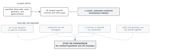
Classification of apparent semiclassical instabilities. The map is schematic and not to scale; retarded support, Ward identities, gauge invariance, and the EFT frequency bound precede any physical stability conclusion.

Domain and failure conditions

See the chapter domain and failure-conditions table. The criterion assumes a self-consistent background, a Hadamard state, a retarded renormalized kernel, compatible state perturbations, and a controlled gauge/constraint reduction. It must be weakened for secularly changing backgrounds, nonstationary kernels, infrared nonuniformity, or frequencies near the EFT cutoff. Bounded mean response does not bound stress variance or induced metric fluctuations.

Exercise

With the Fourier convention above, classify the time dependence from poles at $\omega=\Omega-i\gamma$, $\omega=i\gamma$, and $\omega=M_*$, where $\gamma>0$ and $M_*$ is the EFT cutoff.

Solution

The first gives $e^{-i\Omega t}e^{-\gamma t}$ and decays. The second gives $e^{+\gamma t}$ and grows, subject to gauge and constraint checks. The third is oscillatory but lies at the cutoff; the truncated EFT does not license it as a physical mode merely because it is bounded.

References

• Anderson, P. R., C. Molina-París, and E. Mottola. “Linear Response, Validity of Semiclassical Gravity, and the Stability of Flat Space.” Physical Review D 67 (2003): 024026. DOI.
• Hu, B. L., and E. Verdaguer. “Stochastic Gravity: Theory and Applications.” Living Reviews in Relativity 11 (2008): 3. DOI.
• Meda, P., and N. Pinamonti. “Linear Stability of Semiclassical Theories of Gravity.” Annales Henri Poincaré 24 (2023): 1211–1243. DOI.