Self-Consistent State–Geometry Solutions

A self-consistent semiclassical solution is a pair $(g,\omega)$ for which the state is defined and admissible on $g$, its renormalized stress is evaluated on $g$, and that same metric satisfies the sourced equation with the declared boundary data and finite couplings. Computing $\langle T_{\mu\nu}\rangle$ on a seed and perturbing a parameter once is only the first iterate unless a controlled perturbative argument closes the loop.

Required background. Coupled initial data supplies admissible state–geometry data; constraints and conservation supplies compatibility; and Hadamard-state construction supplies the state on each candidate metric.

Helpful background. Mode-sum renormalization supplies a source calculation, and EFT breakdown diagnostics fixes the allowed branch and curvature range.

A fixed point in state–geometry space

Let $\mathcal S[g,\omega]$ denote the renormalized semiclassical residual and $\mathcal Q[g]$ the rule that constructs a state from fixed physical boundary and initial data. Self-consistency requires

$$\mathcal S[g,\omega]=0, \qquad \omega=\mathcal Q[g].$$

An iteration is therefore

$$g^{(n)} \xrightarrow{\ \mathcal Q\ } \omega^{(n)} \xrightarrow{\ \langle T\rangle_{\rm ren}\ } T^{(n)} \xrightarrow{\ \mathcal G\ } \widetilde g^{(n+1)},$$

followed, when necessary, by under-relaxation

$$g^{(n+1)} =(1-\lambda)g^{(n)} +\lambda\widetilde g^{(n+1)}, \qquad 0<\lambda\le1.$$

The map $\mathcal Q$ must hold fixed physical data, not coordinate labels that change meaning with $g$. Examples are a proper cavity radius and local temperature, an asymptotic state and mass, or Cauchy two-point data transported by a declared rule. A different boundary condition at every iterate defines a different problem.

Convergence of metric components is insufficient. At the candidate limit verify:

$$\|\mathcal S[g,\omega]\|<\varepsilon_{\rm eq}, \quad \|\nabla^\mu\langle T_{\mu\nu}\rangle\|<\varepsilon_{\rm cons}, \quad \|\mathcal C\|+\|\mathcal C_i\|<\varepsilon_{\rm con},$$

as well as state positivity, Hadamard structure, boundary regularity, and cutoff ratios. The norms and sampling region must be stated; a residual small only in a coordinate component can hide a horizon or boundary singularity.

The structure map ends at this joint fixed point. Every earlier box is recomputed on the candidate geometry rather than inherited unchanged from the seed.

Fixed-point meaning of a self-consistent mean geometry. The diagram is schematic and not to scale; state admissibility, causal prescription, higher-derivative branch, and constraints are tested at the converged pair.

The failure map’s final witness rules out “one-way” calculations. A small correction computed on $g^{(0)}$ is licensed perturbatively only when the omitted reevaluation changes the result beyond the retained order.

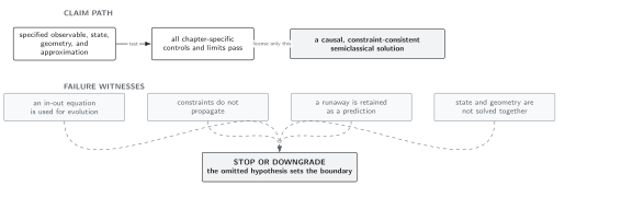
Self-consistency failure and its perturbative exception. This schematic, not-to-scale map permits a one-step result only with an explicit order estimate showing that the next source update is higher order.

Application: a static spherical iteration

Consider a static cavity with

$$ds^2=e^{2\psi(r)}F(r)dt^2 -\frac{dr^2}{F(r)} -r^2d\Omega_2^2, \qquad F(r)=1-\frac{2m(r)}{r}.$$

Fix the induced metric and a local thermal state at the cavity wall. For each $(m^{(n)},\psi^{(n)})$:

1. construct the corresponding regular static Hadamard state with that wall temperature;
2. compute $\rho^{(n)}=\langle T^t{}_t\rangle_{\rm ren}$ and radial pressure $p_r^{(n)}=-\langle T^r{}_r\rangle_{\rm ren}$ with the same finite couplings, using a conserved static mode-sum construction such as Anderson, Hiscock, and Samuel 1995, §§ II–III;
3. solve, at Einstein order,

$$\frac{dm^{(n+1)}}{dr} =4\pi r^2\rho^{(n)}(r), \qquad \frac{d\psi^{(n+1)}}{dr} =\frac{4\pi r[\rho^{(n)}+p_r^{(n)}]}{F^{(n+1)}},$$

with curvature-squared contributions restored or order reduced according to the chosen prescription; 4. normalize $t$ by the wall proper time and under-relax if required.

Convergence is checked in invariant functions such as the Misner–Sharp mass, local Tolman temperature, and orthonormal stress components. It must also be stable under mode cutoff, radial mesh, subtraction implementation, and $\lambda$. A contractive iteration proves convergence of that numerical map, not uniqueness of all semiclassical solutions.

Adversarial test: two seeds and two branches

Start once from a weakly curved configuration and once from a compact configuration with the same wall data. Three outcomes have different meanings:

• both runs converge to the same admissible pair: evidence for an attractor in the tested basin;
• they converge to two admissible pairs: evidence for multiple branches, not a numerical failure;
• one develops a horizon singularity, violates the constraint, or loses Hadamard/state regularity: that branch is rejected even if component iterates settle.

Selecting the branch with the smaller equation residual is not enough when both residuals are below tolerance. Physical selection must follow from initial data, thermodynamic ensemble, or stability. Conversely, failure of simple iteration does not prove absence of a solution; it can reflect a noncontractive solver.

The strongest claim reports the branch, basin explored, boundary data, and stability status. A mathematical existence or uniqueness theorem requires stronger hypotheses than numerical convergence.

Domain and failure conditions

See the chapter domain and failure-conditions table. This page licenses a self-consistent pair only when the same physical state rule, couplings, and boundary data are used throughout, all tensor and constraint residuals converge, and the final state is admissible. It does not infer fluctuation control or nonlinear uniqueness from mean fixed-point convergence; those require stress correlations beyond the one-point source (Hu and Verdaguer 2020, chs. 6–8).

Exercise

If the linearized update has error $e_{n+1}=qe_n$ with $q>1$, find a relaxation range that makes the scalar iteration contractive.

Solution

Under relaxation,

$$e_{n+1}=[(1-\lambda)+\lambda q]e_n.$$

For real $q>1$ and $0<\lambda\le1$, the factor is greater than one, so positive under-relaxation cannot make this mode contractive. One needs a different preconditioner, Newton step, or branch parameterization. Under-relaxation helps oscillatory modes with negative $q$, not every divergence.

Handoff

Quantum-state evolution on backreacted backgrounds treats the time-dependent version, where the state carries memory rather than being reconstructed from static symmetry at every step.

References

• Anderson, Paul R., William A. Hiscock, and David A. Samuel. “Stress-Energy Tensor of Quantized Scalar Fields in Static Spherically Symmetric Spacetimes.” Physical Review D 51 (1995): 4337–4358. doi:10.1103/PhysRevD.51.4337.
• Hu, Bei-Lok, and Enric Verdaguer. Semiclassical and Stochastic Gravity: Quantum Field Effects on Curved Spacetime. Cambridge: Cambridge University Press, 2020. doi:10.1017/9780511667497.