Interacting Scalar Theory on a Curved Background: Benchmark Ledger

This benchmark computes the one-loop two-point correction of a real $\phi^4$ theory on an ultrastatic curved background. The calculation is analytic up to a spectral sum: it fixes the state, Hadamard subtraction, curvature counterterms, kernel convention, and error order, then shows how the result translates under changes of state, renormalization scale, and curvature convention. It is a bounded test, not a theorem for all interacting fields.

Required background. Curved-space time-ordered products supplies the perturbative kernel, curvature counterterms and operator mixing supplies the finite basis, and constructing Hadamard states supplies the ultrastatic reference state.

Helpful background. Running curvature couplings controls scale translation, while schemes and finite parts clarifies which constants must be matched.

Fixture and conventions

Let $M=\mathbb R\times\Sigma$ with

$$ds^2=dt^2-h_{ij}(x)dx^idx^j,$$

where $(\Sigma,h)$ is smooth and compact without boundary. Use

$$S=\int d\mu_g\left[ \frac12(\nabla\phi)^2 -\frac12(m^2+\xi R)\phi^2 -\frac{\lambda}{4!}\phi^4 \right], \qquad P=\Box+m^2+\xi R.$$

The site curvature convention makes $\xi=-1/6$ conformal in four dimensions. Assume the spatial operator

$$A=-\Delta_h+m^2+\xi R$$

is strictly positive. Let $Au_j=\omega_j^2u_j$ with $\omega_j\geq\omega_{\min}>0$ and orthonormal $u_j$. The static ground-state two-point function is

$$G^+_\omega(t,x;t',y) =\sum_j\frac{e^{-i\omega_j(t-t')}}{2\omega_j} u_j(x)\overline{u_j(y)},$$

understood distributionally. Positivity of $A$ removes the zero-mode obstruction and this ground state is Hadamard under the standard ultrastatic hypotheses.

Define the renormalized local fluctuation at scale $\mu$ by

$$w_{\omega,\mu}(x)= \lim_{x'\to x} \left[G^+_\omega(x,x')-H^+_\mu(x,x')\right].$$

This is smooth but depends on the state and on the finite normalization of $[\phi^2]$. Fix those finite terms by two renormalization conditions—for example, one flat reference condition for the $m^2$ part and one curved reference condition for the $R$ part.

For the propagator calculation, use the inverse-kernel convention

$$\mathscr G_F=(P+i0)^{-1}, \qquad P_x\mathscr G_F(x,y)=\delta_g(x,y).$$

The time-ordered expectation used by another source may differ by an overall factor of $i$; translating that factor does not change the inverse-operator result below.

The construction map identifies every input the benchmark must exercise: Hadamard spectral data, renormalized products, the local interaction, curvature counterterms, and the final observable. Inspect the dashed infrared qualification as well—the positive spectral gap is what keeps that separate failure mode outside this fixture.

Construction path exercised by the one-loop scalar fixture. The map is schematic and not to scale; the assumed positive spatial spectrum bounds the infrared question but does not prove an infinite-volume limit.

The validity map turns the benchmark into a falsifiable comparison. State, scale, geometry, and approximation are specified first; a failed translation or field-equation check forces a downgrade rather than being hidden by numerical agreement.

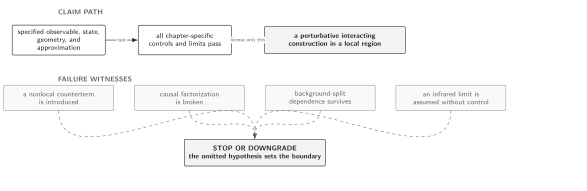
Validity path for the ultrastatic scalar result. This schematic, not-to-scale map makes the first failed translation or control the boundary of the one-loop claim.

One-loop local self-energy

For $\mathcal L_{\rm int}=-\lambda\phi^4/4!$, the one-loop tadpole has symmetry factor $1/2$. After Hadamard subtraction and inclusion of the matter counterterms, its local insertion is

$$M_1^2(x)= \frac{\lambda}{2}w_{\omega,\mu}(x) +\delta m^2(\mu)+\delta\xi(\mu)R(x).$$

Curvature-only counterterms do not enter this fixed-background two-point kernel directly, but they are required if the effective action or stress tensor is also evaluated. Wavefunction renormalization begins beyond this one-loop tadpole in four-dimensional $\phi^4$ theory.

The tadpole’s local form and the need to renormalize the nonminimal and geometric couplings together are derived for curved-space scalar theory in Markkanen and Tranberg 2013, §§ 2–3. Their curvature and Green-function signs must be translated to the conventions fixed above before coefficients are compared.

The corrected inverse kernel is $P+M_1^2+O(\lambda^2)$. The resolvent identity therefore gives the renormalized one-loop answer

$$\boxed{ \mathscr G_{F,\rm R}^{(1)}(x,y) =-\int_M d\mu_g(z)\, \mathscr G_F(x,z)M_1^2(z)\mathscr G_F(z,y) }$$

and

$$\mathscr G_{F,\rm R} =\mathscr G_F+\mathscr G_{F,\rm R}^{(1)}+O(\lambda^2).$$

This is a computation, not merely a counterterm list: once the spectrum $(u_j,\omega_j)$ and the finite renormalization conditions are specified, $w_{\omega,\mu}$ is obtained by a mode sum with local Hadamard subtraction and inserted in the displayed covariant integral.

On a homogeneous ultrastatic space where $R$ and $w_{\omega,\mu}$ are constant, $M_1^2$ is constant and the mode–frequency representation simplifies to

$$\mathscr G_{F,\rm R}^{(1)}(\nu,j) =-M_1^2\,[\mathscr G_F(\nu,j)]^2.$$

Equivalently, it is the first Taylor term of the free propagator with $\omega_j^2\mapsto\omega_j^2+M_1^2$. This provides an independent resolvent check of the combinatorics and sign.

Renormalization and scale check

Changing the Hadamard scale changes the local fluctuation by

$$w_{\omega,\mu'}-w_{\omega,\mu} =a\log\!\frac{\mu'}{\mu} \left[m^2+\left(\xi+\frac16\right)R\right],$$

where $a$ is fixed by the normalization of the parametrix. The running of $\delta m^2$ and $\delta\xi$ cancels this shift in $M_1^2$ through $O(\lambda)$. Thus the corrected two-point function is scale independent to the calculated order after the parameters are translated. Holding the counterterms fixed while changing $\mu$ is an intentionally mismatched comparison.

The local field equation supplies another check:

$$P_x\mathscr G_{F,\rm R}^{(1)}(x,y) =-M_1^2(x)\mathscr G_F(x,y),$$

which follows immediately from $P_x\mathscr G_F(x,z)=\delta_g(x,z)$. A numerical spectral implementation should verify this smeared identity as well as stability under increasing mode cutoff after the Hadamard terms are subtracted.

Adversarial translations

Change the state. For two Hadamard states,

$$w_{\omega',\mu}(x)-w_{\omega,\mu}(x) =\lim_{x'\to x} \left(G^+_{\omega'}-G^+_\omega\right)(x,x')$$

is smooth and generally position dependent. It changes the one-loop self-energy physically. A state-independent counterterm cannot absorb an arbitrary such function. Agreement is expected only after comparing the same transported state or after explicitly predicting the state dependence.

Change the scale. Translate $w$, $m^2(\mu)$, $\xi(\mu)$, and finite insertion constants together. Agreement of $M_1^2$ through $O(\lambda)$ is the check; equality of the unrenormalized coincidence sums is neither expected nor meaningful.

Change the curvature convention. A source using $R_{\rm src}=-R_{\rm site}$ must also use $\xi_{\rm src}=-\xi_{\rm site}$ so that $\xi R$ and $P$ are unchanged. Curvature counterterm coefficients transform with their operators. Comparing printed values of $\xi$ without this translation can turn the conformal value $-1/6$ into an apparent sign error.

Accidental numerical agreement after any one of these changes is not validation. The transformed analytic kernel, renormalization conditions, and residual error order must agree.

Error and validity statement

The chapter domain and failure-conditions table supplies the common comparison. For this fixture, compact boundaryless $\Sigma$, strict positivity of $A$, the static Hadamard ground state, a fixed pair of finite renormalization conditions, and the inverse-kernel convention license the displayed $O(\lambda)$ correction. The decisive checks are the resolvent/field equation and analytic translation under state, scale, and curvature changes. A zero mode blocks the infrared part; unmatched scale or curvature data blocks comparison; and spectral nonconvergence blocks the computed coefficient. In each case the result is downgraded to the largest checked subset rather than extrapolated to a general interacting theory.

Source	Control or bound
Perturbative truncation	Terms omitted from the analytic result are $O(\lambda^2)$ at fixed background, state, and renormalized parameters; no convergence claim is made.
Spectral truncation	Increase the eigenvalue cutoff after subtracting the same number of Hadamard asymptotic terms; require stability of smeared $w_{\omega,\mu}$ and the field-equation residual.
Coincidence extraction	Vary the point-splitting direction inside a convex normal neighborhood; the renormalized scalar limit must agree.
Infrared control	The assumption $\omega_{\min}>0$ is essential. Approaching a zero mode requires a new infrared analysis.
Finite volume and geometry	The result is for the declared compact ultrastatic $\Sigma$; a large-volume or time-dependent limit is a separate claim.
Convention translation	Recompute $P$, $H_\mu$, $\xi R$, and the counterterm basis under any sign or normalization change.

Exercise

Assume $M_1^2$ is constant. Show that the one-loop correction equals the first variation of the free inverse kernel under $m^2\mapsto m^2+sM_1^2$.

Solution

Let $\mathscr G_s=(P+sM_1^2+i0)^{-1}$. Differentiating $(P+sM_1^2)\mathscr G_s=1$ gives

$$\left.\frac{d\mathscr G_s}{ds}\right|_{s=0} =-\mathscr G_FM_1^2\mathscr G_F.$$

In position space this is exactly the covariant convolution displayed above; in the spectral representation it is $-M_1^2\mathscr G_F(\nu,j)^2$.

What the benchmark establishes

Under the ultrastatic, positive-spectrum, Hadamard, local-covariant, and one-loop assumptions, the formula gives a reproducible renormalized scalar two-point correction and passes resolvent, field-equation, scale-translation, and convention-translation checks. It does not establish a nonperturbative interacting state, an adiabatic infinite-volume limit, or a result for arbitrary time-dependent backgrounds.

References

• Hollands, Stefan, and Robert M. Wald. “Quantum Fields in Curved Spacetime.” Physics Reports 574 (2015): 1–35. doi:10.1016/j.physrep.2015.02.001.
• Markkanen, Tommi, and Anders Tranberg. “A Simple Method for One-Loop Renormalization in Curved Space-Time.” Journal of Cosmology and Astroparticle Physics 08 (2013): 045. doi:10.1088/1475-7516/2013/08/045.
• Parker, Leonard, and David J. Toms. Quantum Field Theory in Curved Spacetime: Quantized Fields and Gravity. Cambridge: Cambridge University Press, 2009. doi:10.1017/CBO9780511813924.