Curved-Space Renormalization Schemes: Domains and Translation

Hadamard point splitting, DeWitt–Schwinger expansion, dimensional renormalization, and adiabatic subtraction can represent the same local renormalized observable only on a common domain and after their scales and finite curvature terms are aligned. Their intermediate regulators look different; equality of bare subtractions is neither expected nor required.

Required background. Renormalized Stress Tensor: Axioms and Curvature Ambiguities supplies the allowed finite basis; Adiabatic States, WKB Order, and Regularity distinguishes state regularity; Dimensional Regularization and Minimal Subtraction supplies the pole prescription.

Helpful background. Renormalization Conditions, Schemes, and Finite Parts supplies scheme translation; Asymptotic Scales, Remainders, Uniformity, and Optimal Truncation supplies control of local expansions.

Four prescriptions and one observable

On this page the stress sign is fixed by

$$\delta\Gamma_{\mathrm m} = \frac12\int\mathrm d^4x\,\sqrt{-g}\, \langle T_{\mu\nu}\rangle\,\delta g^{\mu\nu}.$$

Hadamard subtraction removes the local singular biscalar $H_\ell$. DeWitt–Schwinger organizes the same short-distance data through proper time,

$$K(s;x,x') \sim \frac{i\Delta^{1/2}(x,x')}{(4\pi i s)^2} e^{-i\sigma/(2s)} \sum_{n=0}^{\infty}a_n(x,x')(is)^n,$$

with contour and $i0$ data fixed by the propagator. Dimensional renormalization instead isolates local poles at $d=4-2\epsilon$. Adiabatic subtraction expands exact homogeneous modes at large momentum through the order required by the observable.

These constructions share the same ultraviolet locality but not the same automatic domain. DeWitt–Schwinger is a local asymptotic expansion, not a state. Adiabatic subtraction presupposes a mode decomposition and canonical variable. Minimal subtraction fixes poles, not physical finite gravitational couplings.

First application: scalar stress in FLRW

For a spatially flat FLRW metric, rescale a scalar mode to a canonical oscillator,

$$v_{\mathbf k}'' +\Omega_{\mathbf k}^2(\eta)v_{\mathbf k}=0.$$

The adiabatic ansatz

$$v_{\mathbf k}^{(A)} = \frac{1}{\sqrt{2W_{\mathbf k}}} \exp\!\left(-i\int^\eta W_{\mathbf k}(\eta')\,\mathrm d\eta'\right)$$

gives the Riccati equation

$$W_{\mathbf k}^2 = \Omega_{\mathbf k}^2 -\frac12\frac{W_{\mathbf k}''}{W_{\mathbf k}} +\frac34\left(\frac{W_{\mathbf k}'}{W_{\mathbf k}}\right)^2.$$

Iterating in derivatives produces the high-$k$ counterterms. In four dimensions, $\langle\Phi^2\rangle$ requires subtraction through second adiabatic order, while the scalar stress tensor requires fourth order. The original homogeneous-space construction derives the stress subtraction and conservation conditions explicitly Parker and Fulling 1974, §§II–IV, pp. 343–351. The order used to declare an adiabatic state is a regularity property of exact initial data; it is not a license to truncate the stress subtraction at that same number.

Compute the exact-mode stress integrand $t_{\mu\nu,\mathbf k}$ and form

$$\langle T_{\mu\nu}\rangle_{\mathrm{ad}} = \int\frac{\mathrm d^3k}{(2\pi)^3} \left[ t_{\mu\nu,\mathbf k} -t_{\mu\nu,\mathbf k}^{(0-4)} \right].$$

Now compute the point-split result using $H_\ell$. The comparison requires the same $P_\xi=\Box_g+m^2+\xi R$, the same canonical mode normalization, the same metric-variation sign, and a finite shift in the $m^4g_{\mu\nu}$, $m^2G_{\mu\nu}$, $H^{(1)}_{\mu\nu}$, and $H^{(2)}_{\mu\nu}$ basis. Del Río and Navarro-Salas demonstrate the adiabatic–DeWitt–Schwinger equivalence for the stated scalar and spinor settings del Río and Navarro-Salas 2015, §§II–IV. This is not a theorem that adiabatic subtraction is available on every nonhomogeneous spacetime.

Adversarial state-order substitution

Choose a fourth-order adiabatic state and subtract its entire fourth-order approximate two-point function as though it were universal. Depending on the construction, this can import finite state choices and obscure the local scale. Conversely, choose a second-order state and subtract only second order from the stress integrand: quartic, quadratic, or logarithmic ultraviolet terms remain, and conservation can fail after integration.

The strongest surviving statement is a mode-regularized diagnostic until observable-specific ultraviolet order, covariance, and finite translation are verified. A numerical equality of energy density alone is insufficient; pressure, trace, and covariant conservation must agree too.

Translation controls

The structure map shows that equivalent schemes meet only after their local finite terms are classified.

Scheme equivalence is an equality of renormalized observables on a common domain, not an equality of regulators; the map is schematic and not to scale.

The failure map asks first whether the subtraction order belongs to the observable rather than to the state label.

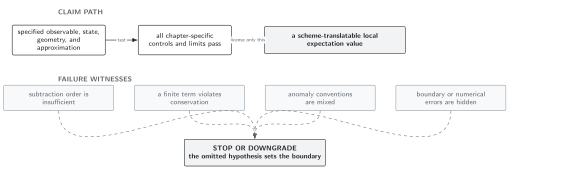
A translated result requires common field conventions, complete ultraviolet order, Ward checks, and explicit finite terms; the map is schematic and not to scale.

Use Domain and failure conditions. Report canonical variables, mode measure, WKB counting, proper-time or dimensional scale, finite coupling map, state, boundary condition, conservation residual, trace convention, and the first neglected asymptotic term.

Mode-Sum and Numerical Renormalization implements analytic subtraction tails. Chapter 2 owns adiabatic state construction; Chapter 8 owns heat-kernel effective actions.

References

• Adrián del Río and José Navarro-Salas, “Equivalence of Adiabatic and DeWitt–Schwinger Renormalization Schemes,” Physical Review D 91 (2015), 064031, DOI, arXiv:1412.7570.
• Leonard Parker and Stephen A. Fulling, “Adiabatic Regularization of the Energy-Momentum Tensor of a Quantized Field in Homogeneous Spaces,” Physical Review D 9 (1974), 341–354, DOI.