Curved-Spacetime Channel Deployment Contract

A curved-field communication claim becomes meaningful only after every map between preparation and readout has been fixed. The minimal specification names the spacetime and field state, sender and receiver worldlines, localized couplings, clocks, encoding, accessible output algebra, decoding, resource constraint, and performance metric. Omitting any one of these can turn a numerical “fidelity” into a comparison between undefined tasks.

Required background. Completely Positive Maps and Causal Quantum Channels supplies the channel axioms. Algebraic Quantum Channels and Localized Operations identifies operations by spacetime support, and Localized Probe and Detector Models supplies the probe–field interaction.

Helpful background. Detector Response Along Curved and Accelerated Worldlines fixes proper-time response. Switching, Smearing, and Detector Regularization controls ultraviolet and switching effects. Operational Locality and Local Measurement Instruments explain supported interventions and readout.

The deployment data

Take a globally hyperbolic spacetime $(M,g)$ and a real field satisfying

$$P_\xi\Phi=(\Box+m^2+\xi R)\Phi=0.$$

In four dimensions the site’s signed conformal coupling is $\xi=-1/6$. A localized probe $\nu=A,B$ may couple through

$$H_{I,\nu}(\tau_\nu) =\lambda_\nu\chi_\nu(\tau_\nu)\, \mu_\nu(\tau_\nu)\, \Phi(F_\nu,\tau_\nu),$$

where $\chi_\nu$ is compactly supported, $F_\nu$ is a normalized spatial smearing in a specified detector frame, and $\mu_\nu$ is a probe observable. The support region $O_\nu\subset M$, not a coordinate interval alone, determines causal relations. The corresponding local scattering morphism or unitary is meaningful only within the chosen interaction model; pointlike or sudden-switching limits require separate distributional control. A local-measurement construction that respects causal factorization is developed by Fewster and Verch 2020, §§ 3–5.

A reproducible deployment record contains:

1. Background: $(M,g)$, boundary conditions if any, field equation, and a state $\omega$ on the relevant algebra.
2. Laboratories: worldlines or worldtubes, tetrads, proper-time origins, and clock synchronization rule.
3. Interventions: interaction density, coupling strengths, switching, smearing, perturbative or exact regime, and ordering of supports.
4. Code: input system, message ensemble, map $\mathcal E_A$, and any reference system used to test entanglement fidelity.
5. Access: a receiver algebra $\mathcal A_B^{\rm acc}$ or an explicitly normalized set of decoded modes; inaccessible modes must be identified rather than inferred from a drawing.
6. Task and resources: decoder $\mathcal D_B$, number of uses, assistance, error criterion, energy Hamiltonian, bandwidth, interaction time, and backreaction tolerance.

The channel is then a map on a declared input state space,

$$\mathcal N_{A\to B}(\rho_A) =\mathcal D_B\!\left[ \operatorname{Res}_{\mathcal A_B^{\rm acc}} \bigl(\mathcal S_B\circ\mathcal S_A\bigr)_* (\rho_A\otimes\sigma_B\otimes\omega) \right].$$

The restriction symbol is deliberately algebraic. It may be represented by a partial trace only after a subsystem factorization or split construction has been supplied.

Static two-probe application

Let

$$ds^2=N^2(\mathbf x)dt^2-h_{ij}(\mathbf x)dx^i dx^j$$

be static, with probes held at $\mathbf x_A$ and $\mathbf x_B$. Their proper times satisfy $d\tau_\nu=N_\nu dt$. Choose smooth compact switchings with $O_B$ to the causal future of $O_A$, and use a finite-width wavepacket code $a_u$ supported by the sender coupling. For a binary coherent code, $\mathcal E_A$ prepares $|+\alpha\rangle_u$ or $|-\alpha\rangle_u$ with equal prior probability. The receiver couples to a mode $v$ defined in its local tetrad and measures a declared quadrature POVM.

At weak coupling, the receiver mean shifts linearly,

$$\delta\langle Q_B\rangle_s =s\,\lambda_A\lambda_B\alpha\,K_{BA}+O(\lambda^3), \qquad s=\pm1,$$

where $K_{BA}$ is an integral of switching, smearing, detector response, and the retarded kernel. The receiver variance contains its preparation noise and the state-dependent field covariance. These are separate reported quantities: $K_{BA}$ is causal gain, while the covariance determines added noise.

For an energy constraint, choose the sender’s local Hamiltonian $H_A=\Omega_A a_u^\dagger a_u$ and require $\operatorname{Tr}(H_A\rho_A)\le E_A$. A Killing-energy convention instead weights local frequency by $N_A$; the two conventions may be translated, but not silently exchanged. State the decoding error, for example the Helstrom error for the two receiver outputs,

$$p_{\rm err}^{\star}=\frac12\left(1-\frac12 \lVert\rho_B^{(+)}-\rho_B^{(-)}\rVert_1\right).$$

This completes the first application: every factor entering the result can be changed independently and reproduced.

The undefined-task test

Now retain the same number labeled “fidelity” but delete $\mathcal A_B^{\rm acc}$. There is no longer a specified output system on which either the decoded state or the comparison state lives. Alternatively, delete the energy constraint and optimize a bosonic code over arbitrarily energetic inputs; the optimization no longer describes the original finite-resource protocol. In the first case no channel task survives. In the second, fixed-code one-shot performance may survive, but an optimized rate does not.

Domain, limits, and maps

The chapter-wide comparison is Domain and failure conditions. This page licenses a channel statement only for the declared geometry, state, supported interactions, receiver algebra, code, resource set, and approximation order. It does not establish that an idealized detector is an available instrument, that perturbation theory controls strong coupling, or that ignoring backreaction remains valid at arbitrary energy.

The structure map shows where each deployment datum enters. Inspect the path from the localized sender coupling to the receiver algebra: field propagation alone is not yet the task-specific channel.

Geometry, state, localized couplings, access, decoding, and resources jointly define the deployed channel; none is supplied by the word “curved.” Schematic; not to scale.

The failure map makes the adversarial deletion explicit. A performance number without an output algebra or resource model must stop before the channel claim.

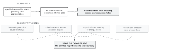
The claimed fidelity or rate is licensed only after the accessible algebra, encoding, decoding, and resource constraint are specified. Schematic; not to scale.

Handoffs

From Propagators and Response Functions to Channel Maps derives the gain and covariance. Causal Channels and Relativistic Communication owns the abstract coding theory, while Energy-Constrained Capacity Under Redshift and Acceleration adds asymptotic rates.

References

• Fewster, Christopher J., and Rainer Verch. “Quantum Fields and Local Measurements.” Communications in Mathematical Physics 378 (2020): 851–889. DOI. Open PDF.
• Martín-Martínez, Eduardo, Miguel Montero, and Marco del Rey. “Wavepacket Detection with the Unruh–DeWitt Model.” Physical Review D 87 (2013): 064038. DOI. Open PDF.