

Langevin and Fokker–Planck Dynamics
The Langevin equation and the Fokker–Planck equation are two representations of one stochastic process only after the time variable, field coordinate, calculus convention, probability measure, drift, diffusion, and boundaries are fixed. For the leading additive de Sitter noise, Itô and Stratonovich agree in ; after a nonlinear field redefinition the required noise-induced drift becomes visible.
Required background. Stochastic coarse-graining derives the scalar coefficients; Langevin fields and noise supplies stochastic conventions; and Fokker–Planck evolution supplies probability currents. Helpful background. Review multiplicative and colored noise.
From an Itô process to probability flow
Section titled “From an Itô process to probability flow”For one field coordinate, write
The Itô density with respect to obeys
where
Normalization changes only by boundary flux: . A reflecting boundary sets ; an absorbing boundary sets the density to zero and intentionally loses survival probability.
For fixed de Sitter and the leading sharp-window scalar coefficients,
so
For a Stratonovich equation with multiplicative coefficient , the equivalent Itô drift is
Likewise, a field change uses Itô’s lemma and adds to the transformed drift. Transforming only the probability curve without its Jacobian and drift changes the process.
For several fields, this bookkeeping becomes geometric rather than optional. A density written relative to coordinate volume is not the same object as one written relative to the field-space volume . The diffusion tensor, connection-induced drift, and probability current must be transformed together. The one-dimensional additive-noise formulas below avoid that ambiguity deliberately; they must not be copied component by component into a curved target space. An implementation check is to evolve the same scalar density in two smooth coordinates and compare transformed expectations of several test functions, not merely the location of the density maximum.
First application: a quartic spectator
Section titled “First application: a quartic spectator”Take with . The moment hierarchy follows from the Itô generator:
At zero current the normalized stationary density is
and hence
Starobinsky and Yokoyama derive the equilibrium and spectral relaxation problem for light self-interacting scalars Starobinsky and Yokoyama 1994, §§II–IV, Eqs. (2.1)–(4.13). This stationary result assumes fixed , zero current at infinity, and a normalizable potential; it is not yet a finite-duration prediction.
Numerically evolve both the Fokker–Planck density on a symmetric field grid and an Euler–Maruyama ensemble. Compare normalization, , , and the full histogram at several time steps and field cutoffs. Strong trajectory convergence is not required for every observable, but weak moment convergence and agreement with the continuum density are. Rare tails need many more trajectories than the central variance.
The structure map places calculus and measure between the coarse-grained noise and stationary or first-passage observables.

For additive leading de Sitter noise, the diffusion coefficient is ; probability flow and boundary conditions determine normalization and later observables. Schematic; not to scale.
Domain and failure conditions
Section titled “Domain and failure conditions”Use the chapter’s domain table. This page assumes a Markov scalar process and a density with respect to the displayed coordinate measure. Multiplicative noise, curved field space, colored kernels, or constrained variables require the corresponding covariant measure and drift.
Adversarial test. Reparameterize to a nonlinear monotone and switch between Itô and Stratonovich. Include the Jacobian and the drift conversion, then transform the resulting density back to . Moments of scalar functions must agree. Reject a stationary distribution that changes merely because the conversion or probability measure was omitted.
The failure map also rejects simulations whose probability loss is caused by an unintended numerical boundary. Controlled densities pass to stationary and first-passage observables; long-correlated noise passes instead to open-system dynamics.
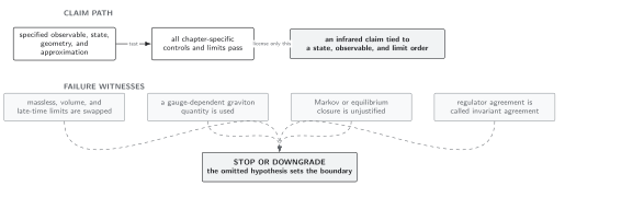
Convention changes leave physical moments invariant only after drift and measure translation; untracked boundary flux invalidates normalization. Schematic; not to scale.
References
Section titled “References”- Starobinsky, A. A., and J. Yokoyama, “Equilibrium State of a Self-Interacting Scalar Field in the de Sitter Background,” Physical Review D 50, 6357–6368 (1994), doi:10.1103/PhysRevD.50.6357.