Covariant Scalar Fields and Curvature Coupling

A real scalar couples to a prescribed curved background through a covariant kinetic term, a mass, and the scalar curvature. Once the metric and curvature conventions are fixed, variation determines the Klein–Gordon operator and the boundary term. The curvature coefficient affects propagation even when gravity is not dynamical; it also controls conformal transport and the improvement term in the classical stress tensor.

This page uses the site’s $(+---)$ metric and curvature convention and writes

$$P_\xi=\Box_g+m^2+\xi R.$$

With this plus-$\xi R$ operator convention, the conformal value is negative:

$$\xi_{\mathrm{conf}} = -\frac{d-2}{4(d-1)}.$$

Equivalently, one may write $P=\Box_g+m^2-\zeta R$ with the common positive parameter $\zeta_{\mathrm{conf}}=(d-2)/[4(d-1)]$. This translation is essential when importing formulas from the literature.

Required background. Curved Spacetimes, Cauchy Surfaces, and Global Hyperbolicity fixes the causal domain; The Klein–Gordon Field and Its Modes supplies the flat-space field and conserved pairing; The Action Principle and Field Equations supplies variational calculus.

Helpful background. Boundaries, Variations, and Well-Posed Actions explains boundary terms; Levi–Civita Connections, Geodesics, and Riemann Curvature fixes the geometric signs.

The curved scalar action

On a $d$-dimensional oriented Lorentzian spacetime, take

$$S[\phi;g] = \frac12 \int_M\mathrm d^dx\,\sqrt{-g} \left[ \nabla_\mu\phi\nabla^\mu\phi -(m^2+\xi R)\phi^2 \right].$$

The combination $\xi R\phi^2$ is local, covariant, and quadratic in the field. In four dimensions $\xi$ is dimensionless, so it is not suppressed as a higher-dimensional interaction. Curved-space renormalization generally requires this coupling even if a special value is imposed at one scale; “minimal coupling” $\xi=0$ is a parameter choice, not a principle protected in every interacting theory Birrell and Davies 1982, §3.1.

Holding the metric fixed and varying $\phi$ gives

$$\begin{aligned} \delta S &= -\int_M\mathrm d^dx\,\sqrt{-g}\, \delta\phi\,P_\xi\phi \\ &\quad +\int_{\partial M}\mathrm d^{d-1}y\,\sqrt{\lvert h\rvert}\, n^\mu\nabla_\mu\phi\,\delta\phi . \end{aligned}$$

The first line follows from

$$\nabla_\mu\phi\,\nabla^\mu\delta\phi = \nabla_\mu\!\left(\delta\phi\,\nabla^\mu\phi\right) -\delta\phi\,\Box_g\phi.$$

This identity also explains why the sign of $\Box_g$ cannot be inferred from a Euclidean formula: it is tied to the Lorentzian action and the declared $(+---)$ metric. The mass and curvature terms contain no derivatives of $\delta\phi$, so they enter the Euler–Lagrange operator with the same plus signs displayed in $P_\xi$.

The bulk equation is therefore

$$(\Box_g+m^2+\xi R)\phi=0.$$

The surface term vanishes for compactly supported variations, suitable falloff, Dirichlet data $\delta\phi|_{\partial M}=0$, or a boundary action and Robin condition chosen to cancel it. It does not vanish merely because the bulk equation holds.

On a Cauchy surface $\Sigma$ with induced volume density $\sqrt h$ and future unit normal $n^\mu$, the canonical momentum density is

$$\pi = \sqrt h\,n^\mu\nabla_\mu\phi.$$

The pair $(\phi|_\Sigma,\pi|_\Sigma)$ gives the freely specifiable scalar data in the boundary-free globally hyperbolic problem. A Robin boundary condition restricts the admissible data at $\partial\Sigma$ and must make the symplectic flux vanish if the bulk theory is to be closed.

The stress tensor requires a local sign declaration. On this page,

$$T_{\mu\nu} = \frac{2}{\sqrt{-g}}\frac{\delta S}{\delta g^{\mu\nu}},$$

which gives positive $T_{00}$ for the minimally coupled scalar in Minkowski space. With the action above,

$$\begin{aligned} T_{\mu\nu} &= \nabla_\mu\phi\nabla_\nu\phi -\frac12g_{\mu\nu} \left[ (\nabla\phi)^2-m^2\phi^2 \right] \\ &\quad -\xi \left[ G_{\mu\nu}\phi^2 +g_{\mu\nu}\Box_g\phi^2 -\nabla_\mu\nabla_\nu\phi^2 \right]. \end{aligned}$$

Its conservation follows from the field equation and the Bianchi identity, subject to the same boundary assumptions used in the variation. Renormalized stress tensors and their finite curvature ambiguity are later constructions.

Two checks fix the interpretation. In Minkowski space with $\xi=0$,

$$T_{00} = \frac12 \left[ (\partial_t\phi)^2 +\lvert\nabla\phi\rvert^2 +m^2\phi^2 \right].$$

For $\xi\ne0$, the extra terms are the curved generalization of the improved stress tensor. They are not an independent force added after solving the field equation: they follow from varying the same metric-dependent action. At the quantum level, the composite stress tensor requires a locally covariant subtraction and admits finite conserved curvature shifts Hollands and Wald 2015, §§3.1–3.2.

Conformal coupling in the site convention

For $m=0$, define

$$L_g = \Box_g-\frac{d-2}{4(d-1)}R.$$

Under $\widetilde g_{\mu\nu}=\Omega^2g_{\mu\nu}$ and

$$\widetilde\phi = \Omega^{-(d-2)/2}\phi,$$

the conformal wave operator obeys

$$L_{\widetilde g}\widetilde\phi = \Omega^{-(d+2)/2}L_g\phi.$$

Thus $L_g=P_\xi$ for $m=0$ and $\xi=\xi_{\mathrm{conf}}$. In four dimensions this is $\xi_{\mathrm{conf}}=-1/6$ in the plus-$\xi R$ notation. If a source calls $+1/6$ “the conformal coupling,” it is normally using $P=\Box+m^2-\zeta R$ or an opposite curvature convention. The invariant round trip is the disappearance of the scale-factor potential for a massless field on a conformally flat spacetime.

The powers of $\Omega$ are fixed, not conventional decoration. The derivative of $\Omega^{-(d-2)/2}\phi$ creates a first-derivative term, while the Weyl transformation of $R$ creates both first- and zeroth-derivative terms. They cancel only for $(d-2)/[4(d-1)]$. A mass term transforms with an extra $\Omega^2m^2$ and therefore breaks this covariance. Birrell and Davies derive the conformal scalar map and its quantum limitations in a convention-translatable form Birrell and Davies 1982, §§3.2 and 6.2.

First application: a scalar in spatially flat FLRW

Use conformal time and

$$\mathrm ds^2 = a(\eta)^2 \left( \mathrm d\eta^2-\mathrm d\mathbf x^2 \right).$$

For any scalar $f$ on this background,

$$\Box_g f = a^{-2} \left[ \partial_\eta^2f +(d-2)\mathcal H\partial_\eta f -\nabla^2f \right].$$

Substituting

$$\phi(\eta,\mathbf x) = \int\frac{\mathrm d^{d-1}k}{(2\pi)^{d-1}}\, \phi_{\mathbf k}(\eta)e^{i\mathbf k\cdot\mathbf x}$$

then gives the mode equation below without assuming a particle interpretation.

For a spatial Fourier mode $\phi_{\mathbf k}$, the equation is

$$\phi_{\mathbf k}'' +(d-2)\mathcal H\phi_{\mathbf k}' +\left(k^2+a^2m^2+a^2\xi R\right)\phi_{\mathbf k} =0, \qquad \mathcal H=\frac{a'}a.$$

Set $v_{\mathbf k}=a^{(d-2)/2}\phi_{\mathbf k}$. In four dimensions,

$$v_{\mathbf k}'' +\left[ k^2+a^2m^2 +a^2(\xi-\xi_{\mathrm{conf}})R \right]v_{\mathbf k} =0.$$

For the site curvature convention, $R=-6a''/a^3$ in four-dimensional spatially flat FLRW. Substituting $\xi_{\mathrm{conf}}=-1/6$ verifies the equation directly. At $m=0$ and $\xi=\xi_{\mathrm{conf}}$, $v_{\mathbf k}''+k^2v_{\mathbf k}=0$: the conformal field has been mapped to the Minkowski wave equation.

For general parameters define the time-dependent squared frequency

$$\omega_{\mathbf k}^2(\eta) = k^2+a^2m^2 +a^2(\xi-\xi_{\mathrm{conf}})R.$$

This quantity can become negative for some modes without making the original action ill-defined; it signals a growing or nonoscillatory interval in the chosen mode variable and demands a stability and state analysis. Conversely, $\omega_{\mathbf k}^2>0$ does not select a unique positive-frequency solution when it varies with time.

For two complex solutions, the Klein–Gordon current gives

$$(u,v)_{\mathrm{KG}} = i\int_{\Sigma_\eta}\mathrm d^{d-1}x\, a^{d-2} \left( u^*v'-u^{*'}v \right).$$

For rescaled four-dimensional modes this becomes the conserved Wronskian

$$i\left(v_{\mathbf k}^*v_{\mathbf k}'-v_{\mathbf k}^{*'}v_{\mathbf k}\right).$$

No vacuum has been chosen: the equation and Wronskian determine the classical solution space, not a preferred positive-frequency subspace.

The first adversarial test keeps $a(\eta)$ fixed and changes $\xi$ away from $\xi_{\mathrm{conf}}$. The scale-factor potential returns even at $m=0$, so the conformal Minkowski modes no longer solve the field equation. The second keeps the operator fixed but replaces one normalized complex mode basis by another Bogoliubov-related basis. The Wronskian and commutator remain unchanged while the state and particle interpretation change. Together these tests separate a change of dynamics from a change of representation.

Construction and failure maps

The construction map places the scalar operator and its curvature coupling before the solution space, commutator, and state. Inspect that order when translating a sign convention or rescaling an FLRW mode.

Mass, curvature coupling, causal domain, and boundary data determine the classical scalar system before a vacuum is chosen; the map is schematic and not to scale.

The failure map is applied here by changing one input at a time. A wrong Riemann sign, conformal weight, boundary normal, or Wronskian factor invalidates the claimed scalar transport even if the mode equation looks familiar.

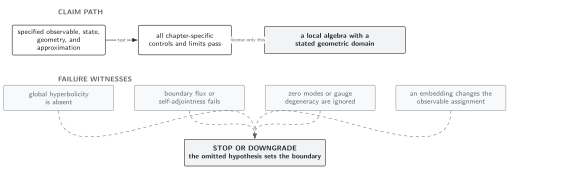
The FLRW and conformal results are licensed only for the declared operator, dimension, boundary problem, and conserved normalization; the map is schematic and not to scale.

The chapter comparison is in Domain and failure conditions. For the scalar, the decisive data are $(m,\xi)$, curvature convention, causal-boundary domain, source support, and conserved pairing; changing any of them requires recomputing the Green operator and algebra.

Convention and boundary checks

• Reversing the Riemann-sign convention sends $R\mapsto-R$ and therefore $\xi\mapsto-\xi$ if $P_\xi$ is to describe the same operator.
• Changing spacetime dimension changes both the field weight and $\xi_{\mathrm{conf}}$.
• A Robin condition $n^\mu\nabla_\mu\phi+\lambda\phi=0$ generally requires a matching boundary term and a specified orientation of $n^\mu$.
• The flat limit $a\to1$, $R\to0$ recovers $\phi_{\mathbf k}''+(k^2+m^2)\phi_{\mathbf k}=0$.

These checks distinguish a convention translation from a physical change in $m$, $\xi$, or boundary data.

Check your understanding

In four-dimensional spatially flat FLRW, show directly that a massless scalar has no scale-factor potential precisely when $\xi=-1/6$ in the plus-$\xi R$ convention.

Solution

The rescaled mode equation is

$$v_{\mathbf k}'' +\left[ k^2+a^2(\xi-\xi_{\mathrm{conf}})R \right]v_{\mathbf k}=0.$$

For a nontrivial FLRW background $R$ is not identically zero, so the curvature term vanishes for every mode only if $\xi=\xi_{\mathrm{conf}}=-1/6$. The result becomes $v_{\mathbf k}''+k^2v_{\mathbf k}=0$, and the inverse rescaling $\phi_{\mathbf k}=a^{-1}v_{\mathbf k}$ returns the conformal solution. A source using $P=\Box-\zeta R$ writes the same condition as $\zeta=+1/6$.

References

• Nicholas D. Birrell and Paul C. W. Davies, Quantum Fields in Curved Space, Cambridge University Press (1982), §§3.1–3.2, DOI.
• Stefan Hollands and Robert M. Wald, “Quantum Fields in Curved Spacetime,” Physics Reports 574 (2015), 1–35, DOI, Open PDF.
• Leonard Parker and David Toms, Quantum Field Theory in Curved Spacetime: Quantized Fields and Gravity, Cambridge University Press (2009), Chapters 2–3, DOI.