Geometric Discretization and Continuum Checks

A curved-space discretization approximates both a field theory and its background geometry. Refining the field variables alone does not define a continuum limit: the metric representation, volume form, curvature coupling, boundary geometry, state, composite subtraction, and physical volume must approach declared targets along the same refinement sequence.

Required background. Mode-Sum and Numerical Renormalization supplies continuum subtraction checks; Lattice Regulators and Target Continuum Theories supplies regulator-to-target matching; Lattice Geometry, Boundaries, and Anisotropy supplies geometric lattice data.

Helpful background. Local Covariance, Isometries, and Background Embeddings supplies comparison maps; Counterterms, Subdivergences, and Locality explains regulator-induced local terms.

Discrete field and geometry as one approximation

On an ultrastatic background, a finite-element scalar discretization has the quadratic action

$$S_h = \frac12\int\mathrm dt\, \left( \dot{\boldsymbol\phi}^{\,T}M_h\dot{\boldsymbol\phi} -\boldsymbol\phi^{T}K_h\boldsymbol\phi \right).$$

The mass matrix $M_h$ approximates $\int_\Sigma\sqrt h\,\phi^2$; the stiffness matrix $K_h$ approximates

$$\int_\Sigma\mathrm d^3x\,\sqrt h\, \left(h^{ij}\nabla_i\phi\nabla_j\phi +(m^2+\xi R)\phi^2\right)$$

with the declared boundary condition. Define

$$\Omega_h^2 = M_h^{-1/2}K_hM_h^{-1/2}.$$

For a positive operator, the discrete ground-state covariance is

$$C_h = \langle\boldsymbol\phi\boldsymbol\phi^T\rangle_h = \frac12M_h^{-1/2}\Omega_h^{-1}M_h^{-1/2}.$$

This formula exposes three different approximations: the geometry and volume in $M_h$, the differential operator and curvature in $K_h$, and the state through the chosen positive-frequency covariance. A graph Laplacian with unit vertex weights generally approximates none of these on an irregular curved mesh.

Raw diagonal entries of $C_h$ diverge as $h\to0$. Define a local observable either as a matched difference on the same mesh or by subtracting a discrete representation of the continuum Hadamard singularity:

$$\mathcal O_h^{\mathrm{ren}}(x_i) = \mathcal D_h \left[C_h-H_h\right]_{ii} +\mathcal O_{h,\mathrm{fin}}(x_i).$$

The derivative operator $\mathcal D_h$, subtraction $H_h$, and finite term must converge to the same continuum prescription. A small discrete field-equation residual does not establish that composite-operator matching.

First application: refined curved meshes

Choose a smooth compact spatial manifold $(\Sigma,h)$ and quasi-uniform triangulations with maximum geodesic edge length $a_n\to0$. For each mesh:

1. construct $M_n,K_n$ from the same piecewise-geometric approximation;
2. verify low generalized eigenvalues $K_n u=\omega_n^2M_n u$ against the continuum spectrum;
3. prepare the same physical Gaussian state;
4. compute a same-background state difference or subtract $H_n$;
5. interpolate the result to common physical points;
6. compare with a continuum mode-sum fixture.

For an observable of engineering dimension $\Delta$, compare the dimensionless quantity $L^\Delta\mathcal O_n$, where $L$ is a fixed physical curvature scale. A controlled refinement fit has the form

$$\mathcal O_n = \mathcal O_{\mathrm{cont}} +A\,a_n^{p_{\mathrm f}} +B\,a_n^{p_{\mathrm g}} +C\,e^{-L_{\mathrm{box}}/\ell_{\mathrm{corr}}} +\cdots .$$

The effective convergence order is limited by both the field order $p_{\mathrm f}$ and geometry order $p_{\mathrm g}$. The finite-volume term is independent of either discretization order. At least three well-separated resolutions are needed to test a proposed power, and removing the coarsest mesh should leave $\mathcal O_{\mathrm{cont}}$ stable within the combined uncertainty.

Use two triangulation families not related by the same local connectivity. Agreement after matching physical points tests restoration of rotational or diffeomorphism covariance more strongly than refinement of one family. On symmetric targets, also monitor multiplet splittings in the low spectrum.

The quantum finite-element proposal combines finite-element weights with simplicial geometry and explicitly anticipates regulator-dependent counterterms Brower et al. 2016, §§2–4, pp. 2–7 of the arXiv PDF. Its interacting curved-sphere implementation demonstrates why those ingredients must be tested together Brower et al. 2018, §§II–IV, pp. 014502-3–014502-12. Those numerical results are model- and manifold-specific evidence, not a theorem that one counterterm set works for every curved theory.

Adversarial false plateau

Refine the field basis while freezing a piecewise-flat geometry whose deficit angles do not converge to the target curvature. Then

$$\lim_{a_{\mathrm f}\to0}\mathcal O(a_{\mathrm f},a_{\mathrm g}^{\mathrm{fixed}}) = \mathcal O_{\mathrm{cont}}[g_{\mathrm{wrong}}],$$

which can form an impressively flat plateau. Likewise, taking $a\to0$ at fixed $L_{\mathrm{box}}$ establishes only a finite-volume continuum result; it does not remove topology or image effects.

Vary $a_{\mathrm f}$, $a_{\mathrm g}$, and $L_{\mathrm{box}}$ independently. A claim about the target infinite-volume curved observable survives only if all three limits are either taken or bounded. If geometry remains fixed, the strongest result is a continuum field theory on the approximating geometry.

Discretization and failure maps

The structure map should be read with the geometry and field branches advancing together toward a common local observable.

Field spacing, geometric approximation, finite volume, and composite renormalization are independent controls; the map is schematic and not to scale.

The failure map identifies a plateau with the wrong geometry or volume as a downgrade, even when the algebraic solver has converged.

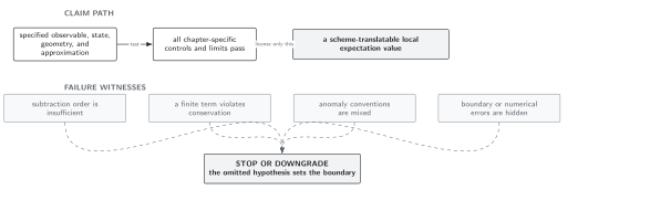
Solver convergence certifies the discrete problem; only matched refinement and continuum fixtures certify the intended curved-space observable; the map is schematic and not to scale.

Use Domain and failure conditions. Report mesh families and quality, physical scale, $M_h,K_h$, curvature and boundary approximation, state preparation, local subtraction, counterterms, interpolation, separate field/geometry/volume limits, fit windows, symmetry restoration, and continuum fixtures.

Check your understanding

Why is agreement of the lowest eigenvalue alone insufficient to validate $C_h(x,x)$?

Solution

The coincident covariance receives contributions from the entire spectrum and is ultraviolet divergent before subtraction. A correct low eigenvalue tests infrared geometry, not the high-mode density or the local composite counterterm.

Boundaries, Surface Counterterms, and Boundary Stress supplies the boundary refinement conditions. Volume VIII owns general lattice universality and extrapolation; implementation-specific claims belong to their executable calculation.

References

• Richard C. Brower, George T. Fleming, Andrew Gasbarro, Timothy G. Raben, Chung-I Tan, and Evan Weinberg, “Quantum Finite Elements for Lattice Field Theory,” Proceedings of Science, LATTICE2015 (2016), 296, DOI, arXiv:1601.01367.
• Richard C. Brower, Michael Cheng, George T. Fleming, Andrew D. Gasbarro, Timothy G. Raben, Chung-I Tan, and Evan S. Weinberg, “Lattice $\phi^4$ Field Theory on Riemann Manifolds: Numerical Tests for the 2D Ising CFT on $\mathbb S^2$,” Physical Review D 98 (2018), 014502, DOI, arXiv:1803.08512.