Higher-Derivative Semiclassical Initial-Value Problems

Renormalizing the mean stress in four spacetime dimensions requires local gravitational couplings beyond $G$ and $\Lambda$. Their metric variations contain up to four derivatives, so treating the resulting equation as exact enlarges its initial-data space and introduces short-scale branches. In an effective field theory, however, those branches generally lie at the cutoff and are not additional particles predicted by the truncated action. The central task is to separate the mathematical initial-value problem from the low-energy predictive problem.

Required background. The semiclassical Einstein equation fixes the mean equation and stress-tensor convention; renormalization of gravitational couplings explains why curvature counterterms are compulsory; and effective field theory as a controlled expansion supplies the low-frequency interpretation.

Helpful background. Constraints, conservation, and Bianchi identities identifies the admissible initial data, while EFT truncation errors and breakdown diagnostics supplies the cutoff tests.

Curvature-squared equations and their data

Use the metric-variation conventions

$$T_{\mu\nu}=\frac{2}{\sqrt{-g}}\frac{\delta S_{\rm m}}{\delta g^{\mu\nu}}, \qquad H^{(i)}_{\mu\nu}=\frac{2}{\sqrt{-g}} \frac{\delta I_i}{\delta g^{\mu\nu}},$$

with, for example,

$$I_1=\int d^4x\sqrt{-g}\,R^2, \qquad I_2=\int d^4x\sqrt{-g}\,R_{\rho\sigma}R^{\rho\sigma}.$$

After fixing the finite couplings, a representative mean equation is

$$G_{\mu\nu}+\Lambda g_{\mu\nu} +a_1H^{(1)}_{\mu\nu}+a_2H^{(2)}_{\mu\nu} =8\pi G\,\langle T_{\mu\nu}\rangle_{\rm ren}.$$

Both $H^{(i)}_{\mu\nu}$ are identically conserved. They include terms such as $\nabla_\mu\nabla_\nu R-g_{\mu\nu}\Box R$, so a direct metric formulation is generically fourth order. The Gauss–Bonnet identity removes one quadratic invariant in four dimensions up to topology and boundary terms, but it does not remove all fourth derivatives.

For an unconstrained fourth-order ordinary equation, one supplies $q$, $\dot q$, $\ddot q$, and $q^{(3)}$ on the initial slice. In gravity, diffeomorphism constraints and gauge equivalence reduce the freely specifiable data, yet they do not turn a generic curvature-squared equation back into a second-order one. Boundary terms must also be handled if the variational problem itself is posed on a finite region.

The structure map locates the key interpretive choice: the same local terms are required for renormalization, but the high-frequency solutions of the truncated equation are accepted or excluded according to the declared theory and scale hierarchy.

Higher derivatives in the semiclassical mean equation. The map is schematic and not to scale; the Bianchi constraints apply to every branch, while EFT control additionally restricts frequencies and curvatures below the cutoff.

Characteristic branches in a linear model

The simplest faithful model is

$$\ddot q+\omega_0^2q=s\,\varepsilon q^{(4)}, \qquad 0<\varepsilon\omega_0^2\ll1, \qquad s=\pm1.$$

For $q=e^{\lambda t}$, the characteristic equation is

$$s\varepsilon\lambda^4-\lambda^2-\omega_0^2=0.$$

Writing $y=\lambda^2$ gives

$$y_\pm=\frac{1\pm\sqrt{1+4s\varepsilon\omega_0^2}} {2s\varepsilon}.$$

One pair is continuously connected to the two-derivative solution,

$$y_-=-\omega_0^2+s\varepsilon\omega_0^4+O(\varepsilon^2).$$

The other has $\lvert y_+\rvert\sim\varepsilon^{-1}$. For $s=+1$ it is exponentially growing or decaying; for $s=-1$ it is a rapid oscillation. Either way its characteristic frequency is $\Omega_{\rm high}\sim\varepsilon^{-1/2}$, precisely where a derivative expansion that retained only the $O(\varepsilon)$ operator is no longer ordered.

This model captures two distinct statements. Mathematically, the full fourth-order equation needs additional initial data and admits the high-frequency pair. Predictively, a low-energy EFT supplies only data analytic in $\varepsilon$ and resolves histories with $\omega\sqrt{\varepsilon}\ll1$; it cannot assign physical significance to a branch whose derivatives make every omitted higher operator equally important. Simon made this distinction explicit for semiclassical gravity and perturbative constraints (Simon 1990, §§ II–III).

Linearized semiclassical application

Let $g_{\mu\nu}=\bar g_{\mu\nu}+h_{\mu\nu}$ about a self-consistent background. After gauge fixing and solving the linearized constraints, a physical polarization schematically satisfies

$$\mathcal D_2 h +\frac{c_4}{M_*^2}\mathcal D_4 h +8\pi G\int dV_y\,\Pi^{\rm ret}(x,y)h(y)=0.$$

The local fourth-derivative operator and the nonlocal retarded response have different origins and must both be retained at their assigned order. For Fourier scales $\lvert\omega\rvert,\lvert\mathbf k\rvert\ll M_*$, solve perturbatively about the two-derivative branch. If instead initial data are chosen so that $\partial_t^2h\sim M_*^2h$, the nominally suppressed term is order one and all higher-derivative operators allowed by symmetry must be restored.

An adversarial test deliberately excites the $y_+$ mode while decreasing the numerical time step. The solution may converge beautifully as a solution of the truncated fourth-order equation. It nevertheless fails the EFT test because its frequency remains of order $M_*$ and the ratio of successive derivative terms does not decrease. Numerical solvability is not low-energy predictivity.

The failure map highlights this branch test. The relevant question is not whether the extra solution exists algebraically, but whether the assumptions used to truncate the action license it.

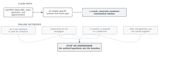
Failure conditions for a higher-derivative initial-value problem. The diagram is schematic and not to scale; a grid-convergent cutoff-frequency branch fails the derivative-expansion control even when it satisfies the truncated equation exactly.

Domain and failure conditions

See the chapter domain and failure-conditions table. A fourth-order formulation is meaningful only after the finite curvature couplings, boundary conditions, gauge, constraints, state, and interpretation of the truncated action are declared. Its low-energy predictions fail when characteristic frequencies or curvature invariants approach the suppression scale, when omitted operators are not smaller, or when extra initial data select a branch nonanalytic in the EFT coefficients.

Exercise

For the linear model with $s=+1$, show that setting the amplitudes of the two high-frequency exponentials to zero leaves a two-dimensional solution space with a perturbatively shifted oscillation frequency.

Solution

The high root is $y_+=\varepsilon^{-1}+\omega_0^2+O(\varepsilon)$ and produces $e^{\pm\sqrt{y_+}t}$. Removing both amplitudes leaves the root $y_-=-\omega_0^2+\varepsilon\omega_0^4+O(\varepsilon^2)$. Hence

$$q(t)=A\cos(\omega_{\rm eff}t)+B\sin(\omega_{\rm eff}t), \qquad \omega_{\rm eff}=\omega_0\left(1-\frac12\varepsilon\omega_0^2\right) +O(\varepsilon^2).$$

Only $A$ and $B$ remain, matching the data count of the low-energy second-order branch.

References

• Horowitz, G. T. “Semiclassical Relativity: The Weak-Field Limit.” Physical Review D 21 (1980): 1445–1461. DOI.
• Parker, L., and J. Z. Simon. “Einstein Equation with Quantum Corrections Reduced to Second Order.” Physical Review D 47 (1993): 1339–1355. DOI.
• Simon, J. Z. “Higher-Derivative Lagrangians, Nonlocality, Problems, and Solutions.” Physical Review D 41 (1990): 3720–3733. DOI.