

Matching Amplitudes to Background Observables
A flat-space amplitude and a weak-background response can encode the same low-energy kernel, but they are not automatically the same observable. Matching requires a common metric normalization, operator basis, source coupling, boundary prescription, and invariant output. Off-shell coefficients may move under gauge choices and field redefinitions even when the scattering amplitude or relational response is unchanged.
Required background. One-Loop Graviton EFT supplies analytic and nonanalytic loop terms; Matching Conditions Beyond Tree Level supplies the matching equation; and Relative Cauchy Evolution and Background Response supplies a local-covariant meaning of metric response.
Helpful background. Curvature Operators and Field-Redefinition Redundancies supplies basis changes, while Gauge-Invariant Response Kernels supplies causal curved-space response.
One kernel, two experimental questions
Section titled “One kernel, two experimental questions”Use and define
Since , the linear coupling is
After gauge fixing and projection onto conserved sources, write the renormalized quadratic action as
Solving gives the linear background response. Eliminating gives the exchange functional
whose cross term between and generates the graviton-mediated amplitude. Thus both calculations use , but the amplitude contracts it with asymptotic states whereas a background experiment evaluates a clock, curvature, trajectory, or flux functional of the solution.
The structure map places an observable dictionary after matching precisely because the metric component remains gauge dependent.

The same inverse quadratic kernel can govern source exchange and linear background response, but external-state normalization and the final invariant observable must be specified separately. The map is schematic and not to scale.
First application: a stationary source
Section titled “First application: a stationary source”Let a conserved compact source be stationary, so , and decompose the projected inverse kernel at low spatial momentum as
Here denotes the conserved-source spin projector, depends on the active loop sectors and normalization, and is analytic at . A complete one-loop source amplitude also receives vertices, boxes, and nonlinear source couplings. For two massive sources it can be organized schematically as
The classical square-root and quantum logarithm have different origins and coefficients; both are dimensionless relative corrections in the displayed normalization. Their full coefficients are matched from the complete effective action rather than attributed to the two-point kernel alone. Local terms in and are retained in both descriptions under one renormalization convention. The separation of long-range nonanalytic pieces from local terms is developed in Donoghue 1994, §§III–IV, pp. 3878–3884.
To turn the solution into a weak-background observable, place two matter-defined worldlines and compare their clock frequencies, or evaluate a tidal component in their transported tetrad. For a static gauge used only as an intermediate calculation,
The operationally reported quantity is the contraction at the event selected by the matter apparatus, not the coordinate component alone. Its far-zone tail follows by Fourier transforming the nonanalytic terms. Boundary conditions must also match: an in–out amplitude uses Feynman boundary values, whereas a causal forced background requires the corresponding retarded kernel.
Field-redefinition adversarial test
Section titled “Field-redefinition adversarial test”Apply
The quadratic kernel, the coefficients of Ricci operators, and the coordinate expression for change. The matter action simultaneously generates contact interactions and changes the dictionary between the field variable and the metric measured by rods and clocks. When all induced terms are retained, the on-shell amplitude is invariant by the equivalence theorem Kamefuchi, O’Raifeartaigh, and Salam 1961, pp. 529–535, and the relational background observable agrees to the matched order.
Comparing only the transformed , or transforming the gravitational action without its source coupling, fails this test. A residual difference after the complete transformation is a useful estimate of omitted EFT order only if it scales with the declared remainder; otherwise it signals inconsistent matching.
Where the dictionary stops
Section titled “Where the dictionary stops”A generic curved spacetime need not possess asymptotic particle states, so no flat-space S-matrix is presumed there. One may still match local Wilson coefficients in a small-curvature expansion and compute causal, relational observables, but global particle-production or horizon questions require their own state and boundary data. Conversely, a flat-space amplitude cannot determine coefficients that vanish on shell yet affect a sourced background unless the matching set includes an appropriate observable.
Domain and failure conditions
Section titled “Domain and failure conditions”The chapter comparison table requires the field normalization, local basis, gauge, source convention, contour, asymptotic or background domain, and final invariant observable. The weak-background expansion requires curvatures and gradients below the EFT cutoff and a source for which linear response is controlled.
The failure map identifies an untransformed source coupling as the characteristic field-redefinition error.
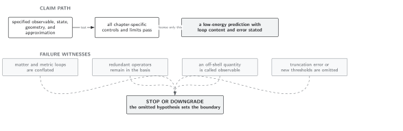
Amplitude-to-background matching fails when field variables, source couplings, boundary prescriptions, or operational observables are compared in different conventions. The map is schematic and not to scale.
References
Section titled “References”- Donoghue, J. F. “General Relativity as an Effective Field Theory: The Leading Quantum Corrections.” Physical Review D 50, 3874–3888 (1994). doi:10.1103/PhysRevD.50.3874. Open PDF
- Kamefuchi, S., L. O’Raifeartaigh, and A. Salam. “Change of Variables and Equivalence Theorems in Quantum Field Theories.” Nuclear Physics 28, 529–549 (1961). doi:10.1016/0029-5582(61)90056-6