Relational and Gauge-Invariant Gravitational Observables

A coordinate value such as $h_{00}(t,\boldsymbol x)$ is not a gravitational observable until the event, frame, and measuring apparatus are specified without relying on the gauge labels being tested. Perturbative relational observables do this by using dynamical clock and rod fields, asymptotic structures, or invariantly defined geometric events. Their construction is order dependent and must be transformed together with the EFT field basis.

Required background. Background-Field Quantization, Gauge Fixing, and Ghosts supplies gauge transformations; Gauge-Invariant Response Kernels supplies invariant linear response; and Local Covariance, Isometries, and Background Embeddings supplies the local-covariant setting.

Helpful background. Gauge, BRST, and BV Interfaces on Curved Backgrounds supplies the interacting gauge complex, while Matching Amplitudes to Background Observables supplies the field-basis dictionary.

Four reference fields and an inverse map

Let four scalar matter fields $X^A$, $A=0,1,2,3$, have background values $X_0^A(x)$ with nonsingular Jacobian in a region:

$$J^A{}_\mu=\partial_\mu X_0^A, \qquad e_A{}^\mu J^B{}_\mu=\delta_A{}^B.$$

Write $X^A=X_0^A+\kappa\chi^A$ and a scalar geometric quantity $\mathcal A=\mathcal A_0+\kappa\,\delta\mathcal A$, where $\kappa$ is a perturbative bookkeeper. The event $x^\mu(X)$ is defined by inverting the four reference fields. To first order,

$$x^\mu(X) =x_0^\mu(X)-\kappa e_A{}^\mu\chi^A,$$

so the relational perturbation at fixed reference values is

$$\delta\mathcal A_{\mathrm{rel}}(X) =\delta\mathcal A -\chi^A e_A{}^\mu\partial_\mu\mathcal A_0.$$

Choose the active gauge convention

$$\delta_\xi(\delta\mathcal A) =\xi^\mu\partial_\mu\mathcal A_0, \qquad \delta_\xi\chi^A =\xi^\mu\partial_\mu X_0^A.$$

The two terms in $\delta\mathcal A_{\mathrm{rel}}$ then cancel exactly. This proof also exposes the domain: the reference-field Jacobian must be invertible, the same gauge sign must be used throughout, and the construction is valid only through the retained perturbative order. Dittrich develops complete observables from clock variables in Dittrich 2006, §§3–5, pp. 6162–6177.

One clock $X$ and a chosen flow $K^\mu$ would give

$$\delta\mathcal A_X =\delta\mathcal A -\frac{\delta X}{K^\mu\nabla_\mu X_0} K^\nu\nabla_\nu\mathcal A_0.$$

That expression is invariant only against gauge displacements along $K^\mu$, or under an explicit gradient-alignment restriction. A generic spacetime diffeomorphism requires enough clock and rod fields to resolve all relevant directions.

The structure map carries a gauge-fixed calculation into this relational completion before making a physical claim.

Reference-field fluctuations shift the event at which a geometric scalar is evaluated, cancelling the gauge shift of the raw perturbation when the reference map is nonsingular. The map is schematic and not to scale.

First application: curvature at a matter-clock event

Take $\mathcal A[g]$ to be a curvature scalar or a tidal scalar formed from the Riemann tensor and a matter-defined tetrad. Compute its renormalized one-loop perturbation in two metric gauges:

$$\delta\mathcal A^{(2)} =\delta\mathcal A^{(1)} +\mathcal L_\xi\mathcal A_0, \qquad \chi_{(2)}^A =\chi_{(1)}^A +\mathcal L_\xi X_0^A.$$

Substitution gives

$$\delta\mathcal A_{\mathrm{rel}}^{(2)} -\delta\mathcal A_{\mathrm{rel}}^{(1)} =\xi^\mu\partial_\mu\mathcal A_0 -\xi^\mu\partial_\mu X_0^A e_A{}^\nu\partial_\nu\mathcal A_0 =0.$$

This is more than an algebraic cancellation. The clock and rod two-point functions, their counterterms, and correlations with the metric must be included at the same loop order. Treating $X^A$ as labels in one gauge but as fluctuating matter in another changes the experiment.

Now perform a local metric redefinition,

$$g_{\mu\nu}'=g_{\mu\nu} +aR_{\mu\nu}+bRg_{\mu\nu}.$$

The coordinate expression for $\mathcal A[g]$, the action of the reference fields, and contact terms all change. Define the primed observable by matching the same apparatus response, not by simply replacing $g$ with $g'$ in one formula. The two descriptions then agree through the matched EFT order; an unmatched raw curvature component need not. In locally covariant perturbative gravity, scalar reference fields provide a concrete way to build such diffeomorphism-invariant functionals Brunetti, Fredenhagen, and Rejzner 2016, §§3–4, pp. 752–768.

Other admissible outputs

In asymptotically flat settings, scattering amplitudes and asymptotic charges can be invariant outputs once their dressing, boundary conditions, and infrared prescription are specified. On a background with distinguished worldlines, clock ratios, radar distance, geodesic deviation, and tetrad-projected curvature are operational alternatives. None licenses a strictly local gauge-invariant metric operator at an arbitrary coordinate point.

Relational observables are not automatically ultraviolet finite. Coincident composite fields still require renormalization, and the reference fields introduce their own fluctuations and possible degeneracies. Nor are they globally complete: caustics or repeated clock values can make $X_0^{-1}$ multivalued.

Coordinate-component adversarial test

Compute $h_{00}(x)$ in two gauges at the same numerical coordinate $x$. Agreement can be accidental and disagreement can be pure gauge; neither has invariant meaning because the two labels need not denote the same physical event. Repeating the comparison at fixed $X^A$ and in the transported matter frame is decisive. Any remaining gauge dependence must be smaller than the declared truncation error or signals an incomplete gauge, counterterm, or reference-field calculation.

Domain and failure conditions

The chapter comparison table requires the gauge convention, reference fields or boundary dressing, invertibility domain, renormalization prescription, field basis, perturbative order, and measured output. A nonperturbative algebra of quantum-gravitational observables and holographic reconstruction lie outside this page.

The failure map highlights singular clock maps and comparisons at fixed coordinate rather than fixed event.

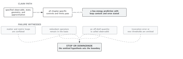
Gauge invariance requires the event and frame to transform with the fields; a singular reference map or an untransformed observable dictionary invalidates the comparison. The map is schematic and not to scale.

References

• Brunetti, R., K. Fredenhagen, and K. Rejzner. “Quantum Gravity from the Point of View of Locally Covariant Quantum Field Theory.” Communications in Mathematical Physics 345, 741–779 (2016). doi:10.1007/s00220-016-2676-x. Open PDF
• Dittrich, B. “Partial and Complete Observables for Hamiltonian Constrained Systems.” Classical and Quantum Gravity 23, 6155–6184 (2006). doi:10.1088/0264-9381/23/22/006. Open PDF