One-Loop Matter Effective Actions in Curved Space

Integrating out a quantum matter field produces a functional of the backgrounds appearing in that field’s Hessian. At one loop this is a determinant, not a quantization of the metric: the geometry is an external argument, and no internal graviton or gravitational-ghost line is included. The central calculation is to separate its local ultraviolet part from finite global, state-dependent, and contour-dependent information.

Required background. The 1PI Effective Action and Mean-Field Equations defines the one-loop Hessian; Gaussian Fields and Sources supplies the determinant from Gaussian integration; and Covariant Scalar Fields and Curvature Coupling fixes the scalar operator and the site’s curvature convention.

Helpful background. Heat Kernels, Zeta Functions, and Spectral Determinants develops the spectral machinery, while In–Out versus In–In Expectation Values distinguishes vacuum amplitudes from causal expectation values.

The matter Hessian and its determinant

Consider a real scalar with Lorentzian quadratic action whose equation is

$$P_\xi\phi=(\Box_L+m^2+\xi R_L)\phi=0.$$

On a smooth Riemannian continuation, declare instead the elliptic operator

$$\mathcal L_E=-\nabla_E^2+m^2-\xi R_E =-\bigl(\nabla_E^2+\xi R_E\bigr)+m^2.$$

This is the convention crosswalk used below. If $\xi_c=-\xi$ is a source’s positive curvature coupling, then $\mathcal L_E=-\nabla_E^2+m^2+\xi_cR_E$. We assume initially a smooth compact manifold without boundary and a positive self-adjoint realization. A kernel is removed explicitly, $\det'\mathcal L_E$; negative modes are excluded from this first calculation because they require a determinant phase.

Expanding about a background matter configuration $\bar\phi$, Gaussian integration gives

$$\Gamma_E[\bar\phi,g_E] =S_E[\bar\phi,g_E] +\frac{\hbar}{2}\operatorname{Tr}'\ln\frac{\mathcal L_E}{\mu^2} +O(\hbar^2).$$

For a complex boson the real-scalar factor $1/2$ changes; for Grassmann fields the determinant enters with the opposite statistics sign. Squaring a first-order Dirac operator determines the modulus but can discard a phase, so that step must be documented separately. These are algebraic consequences of the Gaussian integral, not curvature effects.

First application: the scalar ultraviolet structure

Factor the mass from the heat kernel and write

$$\operatorname{Tr}e^{-s\mathcal L_E} \sim\frac{e^{-m^2s}}{(4\pi s)^2} \int\mathrm d^4x\sqrt{g_E}\, \bigl(a_0+a_1s+a_2s^2+\cdots\bigr).$$

For the scalar convention above,

$$a_0=1, \qquad a_1=\left(\xi+\frac16\right)R_E,$$

and

$$\begin{aligned} a_2={}&\frac1{180} \left(R_{\mu\nu\rho\sigma}R^{\mu\nu\rho\sigma} -R_{\mu\nu}R^{\mu\nu}\right) +\frac12\left(\xi+\frac16\right)^2R_E^2\\ &+\left(\frac1{30}+\frac{\xi}{6}\right)\nabla_E^2R_E . \end{aligned}$$

This follows from the universal Laplace-type coefficients with endomorphism $\mathcal E=\xi R_E$ Vassilevich 2003, Eqs. (2.2), (4.27), and (4.28). It passes the conformal check: $a_1=0$ at $\xi=-1/6$. On a closed manifold the integrated Laplacian is a boundary term; locally, or with a boundary, it must not be dropped.

In dimensional regularization, with the pole convention absorbed into $\bar\epsilon^{-1}$, the local pole is

$$\Gamma_{E,\mathrm{div}}^{(1)} =-\frac{1}{2(4\pi)^2\bar\epsilon} \int\mathrm d^4x\sqrt{g_E}\, \left(\frac{m^4}{2}-m^2a_1+a_2\right).$$

The overall pole sign is tied here to $\Gamma_E^{(1)}=-\tfrac12\int_0^\infty \mathrm ds\,s^{-1}\operatorname{Tr}e^{-s\mathcal L_E}$; counterterms carry the opposite pole. The three mass dimensions match the cosmological, Einstein–Hilbert, and curvature-squared sectors. The finite determinant contains more than these coefficients: large proper time, topology, boundary conditions, and analytic continuation can all matter.

Subtraction-scale and coupling test

Repeat the calculation at $(\xi,\mu)$ and $(\xi+\delta\xi,\mu e^t)$. The pole change is obtained by substituting

$$\delta a_1=\delta\xi\,R_E, \qquad \delta a_2= \left[\left(\xi+\frac16\right)\delta\xi +\frac12(\delta\xi)^2\right]R_E^2 +\frac{\delta\xi}{6}\nabla_E^2R_E.$$

Every ultraviolet change is local and lies in the declared gravitational basis. The scale change likewise moves local logarithms between the determinant and renormalized couplings. A residual nonlocal change caused merely by changing $\mu$ would signal inconsistent subtraction. Conversely, genuinely finite nonlocal form factors cannot be erased by redefining a finite list of local couplings.

The structure map places this determinant before every representation-specific method. Inspect the separation between the Hessian, its domain, and the later heat-kernel, worldline, or nonlocal evaluations.

At one loop the field content and operator domain are fixed before proper time, zeta, or worldline methods are chosen; the metric remains a classical background. Schematic; not to scale.

Domain and failure conditions

This derivation assumes a smooth Euclidean section, a positive self-adjoint scalar operator, declared zero-mode removal, and a local subtraction scheme. A Lorentzian in–out determinant requires an $i0$ prescription and may be complex. A causal stress response requires an in–in contour. The chapter-wide comparison is Domain and failure conditions.

The failure map should be read from its first branch: replacing the matter Hessian by a metric Hessian changes the loop theory, while leaving the operator domain unstated means that no determinant has yet been defined.

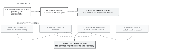
A correct heat-kernel coefficient cannot repair a determinant built from the wrong fluctuating field, boundary condition, kernel, or contour. Schematic; not to scale.

Handoffs

Proper-Time, Zeta, and Determinant Prescriptions defines the spectral representations; Renormalization of Gravitational Couplings by Matter Loops matches the pole; and Matter-Induced Nonlocal Form Factors retains the finite momentum dependence. Graviton and ghost determinants belong to One-Loop Graviton EFT.

References

• Parker, Leonard, and David Toms. Quantum Field Theory in Curved Spacetime: Quantized Fields and Gravity. Cambridge: Cambridge University Press, 2009, chs. 3 and 6. DOI.
• Vassilevich, Dmitri V. “Heat Kernel Expansion: User’s Manual.” Physics Reports 388 (2003): 279–360. DOI. Open PDF.