Order Reduction and Runaway Prescriptions

Order reduction uses the lower-order equations inside perturbatively suppressed higher derivatives, producing an equation with the original data count and the same low-energy solutions through the retained order. It is a controlled effective-field-theory prescription only when the desired solution is analytic in the small coefficients and remains below the derivative cutoff. It is not the same as solving the higher-order equation and imposing a condition in the remote future to cancel its runaway.

Required background. Higher-derivative semiclassical initial-value problems identifies the extra characteristic branches, and EFT truncation errors and breakdown diagnostics supplies the small parameters that license a perturbative replacement.

Helpful background. Effective field theory as a controlled expansion clarifies operator ordering, while constraints, conservation, and Bianchi identities constrains reductions of gravitational equations.

Perturbative reduction of differential order

Consider

$$\ddot q+\omega_0^2q =\varepsilon q^{(4)}+\varepsilon J(t), \qquad \varepsilon\omega_0^2\ll1.$$

For a source family whose derivatives remain bounded as $\varepsilon\to0$, the low-energy branch obeys $\ddot q=-\omega_0^2q+O(\varepsilon)$ and hence

$$q^{(4)}=\omega_0^4q+O(\varepsilon).$$

Substitution on the already $O(\varepsilon)$ right-hand side gives the reduced equation

$$\ddot q+\left(\omega_0^2-\varepsilon\omega_0^4\right)q =\varepsilon J(t)+O(\varepsilon^2).$$

It needs only $q(t_0)$ and $\dot q(t_0)$. The exact homogeneous fourth-order equation instead has

$$\lambda^2+\omega_0^2=\varepsilon\lambda^4,$$

with a low root $\lambda^2=-\omega_0^2+\varepsilon\omega_0^4+O(\varepsilon^2)$ and a runaway root $\lambda^2=\varepsilon^{-1}+O(1)$. The reduced equation reproduces the low root through $O(\varepsilon)$ and never purports to approximate initial data with an order-one runaway amplitude. Parker and Simon implement this logic for one-loop corrected Einstein equations (Parker and Simon 1993, §§ II–IV).

For a tensor equation, reduction must be covariant and constraint compatible. Starting from

$$\mathcal E^{(0)}_{\mu\nu}[g] +\varepsilon\mathcal E^{(1)}_{\mu\nu}[g] =8\pi G\,T_{\mu\nu},$$

one uses $\mathcal E^{(0)}=8\pi GT$ only inside $\varepsilon\mathcal E^{(1)}$. Terms are then rearranged consistently through $O(\varepsilon)$, including derivatives of the source implied by conservation. Reducing only the evolution equations while leaving an unreduced constraint can destroy constraint propagation.

The structure map shows where this prescription acts: after the renormalized, causal mean equation has been obtained, but before cutoff-scale branches are admitted as physical histories.

Order reduction in the semiclassical chain. The map is schematic and not to scale; reduction preserves the retained EFT order only when applied to the full constraint-compatible system and to a causal mean source.

Why a future condition is a different prescription

One can solve the exact fourth-order equation with a retarded source and choose the high-frequency amplitudes so that the growing exponential vanishes as $t\to+\infty$. This “no-runaway” condition uses future information. In simple linear models it rewrites the solution as an integral whose kernel has support slightly before the applied force, producing pre-response on the short scale $\sqrt\varepsilon$.

Order reduction instead defines a local initial-value problem to a specified perturbative order. It changes the differential equation by terms beyond that order and requires no final condition. The two prescriptions can agree in a slowly varying regime up to $O(\varepsilon^2)$, but that agreement is a derived approximation, not an identity. They can differ for rapid sources, transients, nonanalytic initial data, or over times long enough for a formally small difference to accumulate.

In semiclassical gravity a third possibility is to retain a nonlocal form factor whose complete spectral behavior controls the high-frequency response. That is again distinct: one must state the contour, state dependence, and causal kernel rather than infer them from a finite local derivative truncation.

Homogeneous curvature-squared application

Suppose a homogeneous scale variable $q(t)$ represents a gauge-invariant metric perturbation and $\varepsilon q^{(4)}$ comes from a finite curvature-squared coupling. To obtain the one-EFT-order prediction:

1. solve the two-derivative constraint for admissible $q(t_0),\dot q(t_0)$ and state data;
2. replace $q^{(4)}$ using differentiated lower-order evolution and the conserved source;
3. evolve the reduced second-order system with the retarded in-in stress response; and
4. verify $\varepsilon\lvert\partial_t^2\rvert\ll1$ and that the difference between successive truncation orders remains small.

The adversarial data set takes $q^{(2)}(t_0)\sim q(t_0)/\varepsilon$ while keeping $q$ and $\dot q$ modest. It predominantly excites the discarded branch. The reduced equation does not approximate this history; its domain excludes it. Calling the mismatch an “order-reduction error” would reverse the logic of the approximation.

The validity map makes the exclusion explicit. A removed runaway is licensed as an EFT operation only when the retained history independently passes the derivative, constraint, and causal-response checks.

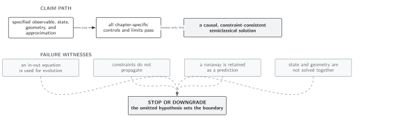
Validity of an order-reduced solution. The diagram is schematic and not to scale; discarded-branch initial data are outside the approximation rather than inaccurately represented within it.

Domain and failure conditions

See the chapter domain and failure-conditions table. Order reduction requires a declared small coefficient, smooth low-frequency data, a solution analytic in that coefficient, and a time interval on which perturbative errors remain uniform. It fails near the cutoff, for branch-dominated initial data, under secular enhancement, or if reduction violates a Ward identity or constraint. A future no-runaway condition must be named separately and checked for pre-response.

Exercise

For $J=0$, compare the low-frequency root of the exact equation with the frequency of the reduced equation through first order in $\varepsilon$.

Solution

The exact low root is $\lambda^2=-\omega_0^2+\varepsilon\omega_0^4+O(\varepsilon^2)$. Writing $\lambda=\pm i\omega_{\mathrm{exact}}$ gives

$$\omega_{\mathrm{exact}}=\omega_0\left(1-\frac12\varepsilon\omega_0^2\right)+O(\varepsilon^2).$$

The reduced equation has $\omega_{\mathrm{red}}^2=\omega_0^2-\varepsilon\omega_0^4$, whose square root is identical through $O(\varepsilon)$. It contains no root of order $\varepsilon^{-1/2}$.

References

• Flanagan, É. É., and R. M. Wald. “Does Back Reaction Enforce the Averaged Null Energy Condition in Semiclassical Gravity?” Physical Review D 54 (1996): 6233–6283. DOI.
• Parker, L., and J. Z. Simon. “Einstein Equation with Quantum Corrections Reduced to Second Order.” Physical Review D 47 (1993): 1339–1355. DOI.
• Simon, J. Z. “Higher-Derivative Lagrangians, Nonlocality, Problems, and Solutions.” Physical Review D 41 (1990): 3720–3733. DOI.