Mukhanov–Sasaki Scalar Modes

The Mukhanov–Sasaki variable is the canonically normalized scalar degree of freedom obtained after the gravitational constraints have been solved. Its oscillator equation makes state normalization, sound-horizon crossing, superhorizon evolution, and the limits of a single-field reduction transparent.

Required background. Gauge-invariant inflationary perturbations fixes the sign of $\zeta$; background symmetry breaking supplies the constrained clock system; and conformal and minimally coupled FLRW scalars supplies the time-dependent oscillator method.

Helpful background. Vacuum choice and initial-state effects explains the ultraviolet condition imposed on the canonical modes.

Constraint reduction and canonical normalization

For a general single-clock theory with scalar sound speed $c_s$, the quadratic curvature action can be written

$$S_\zeta^{(2)}=\frac12\int d\eta\,d^3x\, z^2\left[\zeta'^2-c_s^2(\boldsymbol\nabla\zeta)^2\right], \qquad z^2=\frac{2a^2\epsilon M_{\rm Pl}^2}{c_s^2}.$$

The canonical variable $v=z\zeta$ has action, up to an endpoint term,

$$S_v^{(2)}=\frac12\int d\eta\,d^3x \left[v'^2-c_s^2(\boldsymbol\nabla v)^2+\frac{z''}{z}v^2\right].$$

Each Fourier mode obeys

$$v_k''+\left(c_s^2k^2-\frac{z''}{z}\right)v_k=0, \qquad v_kv_k^{*\prime}-v_k'v_k^*=i.$$

The Wronskian is not an optional normalization convention: it enforces the canonical commutator. A Bogoliubov state changes the positive-frequency solution but must preserve this symplectic product.

The canonical momentum is $\pi_v=v'$, so the Hamiltonian mode by mode is that of an oscillator with time-dependent frequency $\omega_k^2=c_s^2k^2-z''/z$. Positivity of the original kinetic coefficient requires $z^2>0$, and short-wavelength gradient stability requires $c_s^2>0$. A negative $\omega_k^2$ near freeze-out is not a ghost: it describes the ordinary conversion from oscillatory to growing and decaying long-wavelength solutions. A negative kinetic term or ultraviolet $c_s^2$, by contrast, is a genuine instability that cannot be repaired by a state choice.

For constant $\epsilon$ and $c_s=1$, $z''/z=(\nu^2-1/4)/\eta^2$ with

$$\nu=\frac{3-\epsilon}{2(1-\epsilon)}.$$

The adiabatic positive-frequency solution is

$$v_k(\eta)=\frac{\sqrt{-\pi\eta}}{2} e^{i\pi(2\nu+1)/4}H_\nu^{(1)}(-k\eta),$$

which approaches $e^{-ik\eta}/\sqrt{2k}$ at short distance. The reduction and its normalization are given in Garriga and Mukhanov 1999, §§2–3, Eqs. (4)–(15) for general $c_s$.

Long wavelengths and the conserved mode

At $k=0$, the curvature equation integrates exactly:

$$\zeta(\eta)=C_1+C_2\int^\eta\frac{d\eta'}{z^2(\eta')}.$$

In an attractor with growing $a^2\epsilon/c_s^2$, the second term decays and $\zeta$ freezes. This is a dynamical statement, not a consequence of the condition $k=aH$ alone. In an ultra-slow-roll phase, for example, $\epsilon$ falls rapidly and the second solution grows outside the horizon.

The first application is to solve the constant-$\epsilon$ equation, impose the Wronskian, and evaluate $\zeta_k=v_k/z$ at late time. The result supplies the leading scalar spectrum, while the exact Hankel solution quantifies the difference between evaluation at crossing and the asymptotic amplitude. Both normalization and time transport must be retained.

For numerical backgrounds, the same logic gives a robust workflow. Initialize modes only where $c_sk/(aH)$ is large enough that the chosen adiabatic error is below tolerance, evolve the complex mode and its momentum, monitor the Wronskian, and compare the late solution with both the $k=0$ basis and a shifted initialization time. Agreement under that shift tests state preparation; conservation of the Wronskian tests the integrator independently of the power spectrum.

The structure map highlights the passage from constrained variables to one canonical scalar oscillator.

The Mukhanov–Sasaki equation connects canonical short-distance normalization to two long-wavelength solutions; freeze-out follows only when the second solution decays. Schematic; not to scale.

Beyond the one-mode equation

Entropy perturbations add a source to the curvature equation, while rapid changes in $c_s$ invalidate a constant-parameter Hankel approximation. The adversarial test is to compute the nonadiabatic pressure or the turn rate in field space and compare its source term with the nominal decaying mode. If it is not smaller, a single $v$ equation is not closed. Matching across a sharp feature must preserve $\zeta$ and its canonical momentum $z^2\zeta'$ as dictated by the regulated action.

See the chapter’s domain and failure conditions. The validity map marks entropy sourcing, singular $z$, rapid sound-speed evolution, and an incorrectly normalized state as distinct failures.

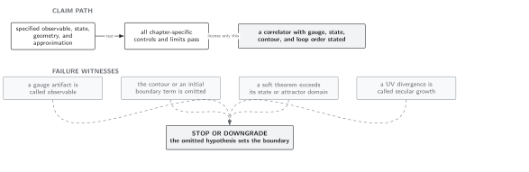
The one-variable equation is controlled only for a regular positive kinetic coefficient, a normalized state, and negligible sources from omitted modes. Schematic; not to scale.

References

• Garriga, J., and V. F. Mukhanov, “Perturbations in $k$-Inflation,” Physics Letters B 458, 219–225 (1999), doi:10.1016/S0370-2693(99)00327-4.
• Mukhanov, V. F., H. A. Feldman, and R. H. Brandenberger, “Theory of Cosmological Perturbations,” Physics Reports 215, 203–333 (1992), doi:10.1016/0370-1573(92)90044-Z.