Gauge-Invariant Response Kernels

A metric response kernel is useful only after diffeomorphism redundancy has been removed without breaking the Ward identities that propagate the gravitational constraints. The safe construction begins with the covariant retarded variation of the renormalized stress tensor, retains its local contact terms, and then projects the coupled metric–state perturbation onto gauge-invariant observables. Gauge fixing may simplify that calculation, but no physical conclusion may depend on the gauge or regulator separately.

Required background. Linear response and semiclassical stability supplies the retarded perturbation equation; constraints, conservation, and Bianchi identities supplies its Ward identities; and relative Cauchy evolution gives the local-algebraic response to compact metric changes.

Helpful background. Gauge, BRST, and BV theory on curved backgrounds organizes gauge independence beyond free metric perturbations, while variation and stress-response consistency fixes contact and counterterm variations.

Scalar gauge invariants on a homogeneous background

For scalar perturbations of a spatially flat FLRW geometry, write

$$ds^2=a^2(\eta)\left[ (1+2A)d\eta^2-2\partial_iB\,d\eta\,dx^i -\left((1-2\psi)\delta_{ij} +2\partial_i\partial_jE\right)dx^idx^j \right].$$

Under the infinitesimal coordinate change generated by

$$\xi^0=T,\qquad \xi^i=\partial^iL,$$

the scalar variables transform as

$$\begin{aligned} A&\longmapsto A-\mathcal HT-T', & B&\longmapsto B+T-L', \\ \psi&\longmapsto\psi+\mathcal HT, & E&\longmapsto E-L, \end{aligned}$$

where $\mathcal H=a'/a$. Thus $\sigma=B-E'$ transforms as $\sigma\mapsto\sigma+T$, and the Bardeen combinations

$$\Phi_{\mathrm B}=A+\sigma'+\mathcal H\sigma, \qquad \Psi_{\mathrm B}=\psi-\mathcal H\sigma$$

are invariant. These definitions use the displayed metric decomposition; changing the sign assigned to $B$ changes intermediate formulas but not invariant observables. Bardeen’s original analysis establishes the scalar-vector-tensor organization and invariant combinations (Bardeen 1980, §§ II–III).

Matter perturbations must be completed in the same way. For a background scalar $\bar\phi(\eta)$,

$$\delta\phi_{\mathrm{gi}}=\delta\phi+\bar\phi'\sigma$$

is invariant with the transformations above. A closed scalar response system is built from $(\Phi_{\mathrm B},\Psi_{\mathrm B},\delta\phi_{\mathrm{gi}})$ together with gauge-invariant state perturbations; the metric potentials alone need not form a closed subsystem.

The structure map should be read from the retarded-response node through the constraint checkpoint. Projection occurs only after the complete covariant variation has been formed.

Gauge-invariant scalar response on a homogeneous background. The map is schematic and not to scale; contact terms and state perturbations are retained before projection, so the gravitational constraints remain part of the physical system.

Covariant kernel and Ward identities

Define the response to a compact contravariant metric perturbation $h^{\rho\sigma}=\delta g^{\rho\sigma}$ by

$$\delta\langle T_{\mu\nu}(x)\rangle_{\mathrm{ren}} =\delta T_{\mu\nu}^{\mathrm{state}}(x) +\int dV_y\, \Pi^{\mathrm R}_{\mu\nu\rho\sigma}(x,y) h^{\rho\sigma}(y).$$

For this inverse-metric variable, its separated-point part is

$$\Pi^{\mathrm R}_{\mu\nu\rho\sigma}(x,y) =+\frac{i}{2}\theta(x\succ y) \langle[T_{\mu\nu}(x),T_{\rho\sigma}(y)]\rangle +\Pi^{\mathrm{contact}}_{\mu\nu\rho\sigma}(x,y).$$

The $+i/2$ follows from the plus source $\frac12\int dV\,h^{\rho\sigma}T_{\rho\sigma}$. If the input is instead the covariant perturbation $\ell_{\rho\sigma}=\delta g_{\rho\sigma}$ used in the displayed FLRW line element, then $h^{\rho\sigma}=-\ell^{\rho\sigma}$ and the response kernel multiplying $\ell$ has separated-point part $-i\langle[T,T]\rangle/2$. The full kernel also includes local variations of the stress operator and finite curvature-counterterm variations. Diffeomorphism covariance does not generally imply the naive equation $\bar\nabla^\mu\Pi_{\mu\nu\rho\sigma}^{\mathrm R}=0$ term by term. Instead the divergence of the full variation vanishes after the variation of the connection acting on the background stress and any state-source term are included:

$$\bar\nabla^\mu\delta\langle T_{\mu\nu}\rangle_{\mathrm{ren}} +(\delta\nabla^\mu) \langle T_{\mu\nu}\rangle_{\mathrm{ren}}=0.$$

This identity is the matter side of the linearized Bianchi identity. A regulator that breaks it must be repaired by allowed local counterterms before the kernel is projected.

Let $Q_A^{\mu\nu}$ denote the differential operators mapping the covariant perturbation $\ell_{\mu\nu}$ to gauge-invariant variables $X_A$, such as $\Phi_{\mathrm B}$ and $\Psi_{\mathrm B}$. The source pullback includes $h^{\mu\nu}=-\ell^{\mu\nu}$, so the projected retarded kernel is symbolically

$$K^{\mathrm R}_{AB} =Q_A\,\Pi^{\mathrm R}\,Q_B^{\dagger},$$

but $Q_B^\dagger$ must act on the constrained source space. Applying a nonlocal scalar-vector-tensor projector without specifying boundary conditions can introduce spurious instantaneous inverse-Laplacian terms. For each nonzero spatial wave number, projection in Fourier space is unambiguous once regularity and boundary conditions are fixed; the homogeneous zero mode must be treated separately as a background variation.

Gauge and regulator adversarial test

Compute the scalar response twice: for example in Newtonian gauge $B=E=0$ and in a regular comoving gauge, using two regulators that preserve locality but may distribute finite contact terms differently. Translate the finite $R^2$ and $R_{\mu\nu}R^{\mu\nu}$ couplings with

$$H^{(i)}_{\mu\nu} =\frac{2}{\sqrt{-g}} \frac{\delta I_i}{\delta g^{\mu\nu}}$$

held fixed as the convention. After solving the same constraints and reconstructing $(\Phi_{\mathrm B},\Psi_{\mathrm B})$, the retarded response to the same gauge-invariant state perturbation must agree. A difference confined to an unprojected variable is gauge; a local polynomial difference accompanied by the translated coupling is scheme; a remaining difference is a failure.

Three independent checks are decisive:

• retarded support: $K^{\mathrm R}_{AB}(x,y)=0$ when $y\notin J^-(x)$;
• constraint consistency: an initially vanishing gauge-invariant constraint residual remains zero to numerical and truncation accuracy; and
• pure-gauge null test: substituting $\ell_{\mu\nu}=2\bar\nabla_{(\mu}\xi_{\nu)}$ produces no invariant response for compactly supported $\xi$.

The failure map makes the order of these checks explicit. Gauge invariance does not rescue an in-out kernel, and retarded support does not rescue a constraint-violating regulator.

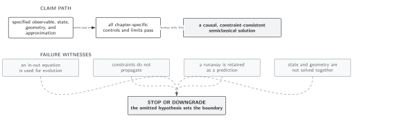
Failure tests for projected metric response. The map is schematic and not to scale; gauge choice and finite renormalization may alter intermediate kernels, but consistently translated gauge-invariant observables must agree.

Domain and failure conditions

See the chapter domain and failure-conditions table. The construction assumes a globally hyperbolic background, specified boundary conditions for scalar projectors, a Hadamard state, a covariantly renormalized retarded kernel, and compatible metric and state perturbations. The $k=0$ sector, backgrounds with boundaries, gauge zero modes, and anomalous Ward identities require separate treatment. This page establishes mean gauge-invariant response, not the gauge-invariant variance of metric fluctuations.

Exercise

Verify the gauge invariance of $\Phi_{\mathrm B}$ and $\Psi_{\mathrm B}$ under the displayed transformations.

Solution

Since $\sigma\mapsto\sigma+T$,

$$\Phi_{\mathrm B}\mapsto A-\mathcal HT-T'+\sigma'+T' +\mathcal H(\sigma+T)=\Phi_{\mathrm B}.$$

Likewise,

$$\Psi_{\mathrm B}\mapsto \psi+\mathcal HT-\mathcal H(\sigma+T)=\Psi_{\mathrm B}.$$

No gauge condition was used.

References

• Anderson, P. R., C. Molina-París, and E. Mottola. “Linear Response, Validity of Semiclassical Gravity, and the Stability of Flat Space.” Physical Review D 67 (2003): 024026. DOI.
• Bardeen, J. M. “Gauge-Invariant Cosmological Perturbations.” Physical Review D 22 (1980): 1882–1905. DOI.
• Kodama, H., and M. Sasaki. “Cosmological Perturbation Theory.” Progress of Theoretical Physics Supplement 78 (1984): 1–166. DOI.