Constraints, Conservation, and the Bianchi Identity

The semiclassical constraints propagate only when the entire renormalized equation is covariantly conserved. The geometric Bianchi identity, matter diffeomorphism Ward identity, nonlocal response contact terms, and boundary fluxes form one compatibility condition. If a regulator leaves a nonconserved source, correcting the geometry after each step hides rather than solves the error.

Required background. The semiclassical Einstein equation defines the residual tensor; conservation and local covariance supplies the renormalized source identity; and stress-tensor Ward identities supplies its symmetry origin.

Helpful background. Interacting stress Ward identities explain contact terms, and variation–response consistency relates the one-point identity to the response kernel.

The compatibility identity

Define the full equation residual

$$\mathcal E_{\mu\nu} =G_{\mu\nu}+\Lambda g_{\mu\nu} +aH^{(1)}_{\mu\nu}+bH^{(2)}_{\mu\nu} -8\pi G\langle T_{\mu\nu}\rangle_{\rm ren}.$$

Each local curvature tensor is the variation of a diffeomorphism-invariant action, so

$$\nabla^\mu G_{\mu\nu}=0, \qquad \nabla^\mu H^{(1)}_{\mu\nu}=0, \qquad \nabla^\mu H^{(2)}_{\mu\nu}=0$$

identically. On the matter equations, invariance of the same renormalized functional gives

$$\nabla^\mu\langle T_{\mu\nu}\rangle_{\rm ren}=0.$$

Therefore $\nabla^\mu\mathcal E_{\mu\nu}=0$. This is not an additional evolution equation; it is the identity that makes four components of $\mathcal E_{\mu\nu}=0$ constraints rather than independent accelerations.

Choose a foliation with normal $n^\mu$ and spatial projector. The Hamiltonian and momentum residuals are

$$\mathcal C=n^\mu n^\nu\mathcal E_{\mu\nu}, \qquad \mathcal C_i=-h_i{}^\mu n^\nu\mathcal E_{\mu\nu}.$$

Projecting $\nabla^\mu\mathcal E_{\mu\nu}=0$ gives a homogeneous first-order system for $(\mathcal C,\mathcal C_i)$ once the spatial evolution equations hold. Hence vanishing constraints on one Cauchy surface remain zero in the continuum problem. Boundary fluxes add explicit source terms and must be included rather than silently set to zero.

For an inverse-metric perturbation $k^{\rho\sigma}=\delta g^{\rho\sigma}$, write the nonlocal response as

$$\delta\langle T_{\mu\nu}(x)\rangle =\int d\mu_y\, \Pi^{\rm R}_{\mu\nu\rho\sigma}(x,y) k^{\rho\sigma}(y) +\delta T^{\rm state}_{\mu\nu}(x),$$

where the separated-point part of $\Pi^{\rm R}$ is $+i\theta\langle[T,T]\rangle/2$ in the site’s plus-source convention. The Ward identity differentiates both the commutator kernel and local contact terms. Transversality of the separated-point commutator alone is insufficient. Christensen’s point-splitting analysis exhibits how covariant subtraction and local geometric terms restore a conserved renormalized stress (Christensen 1976, §§ II–IV).

The structure map’s lower checkpoint points to this chain: causal response and constraint propagation must pass together before stability or self-consistency is interpreted.

Constraint-preserving semiclassical evolution. The diagram is schematic and not to scale; local curvature variations, nonlocal contact terms, initial-state terms, and boundary fluxes all enter the conservation check.

The failure map identifies constraint drift as a physical invalidation, not merely a poor gauge choice. A small spatial evolution residual with growing $\mathcal C$ does not solve the full tensor equation.

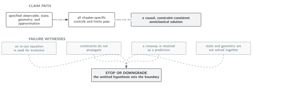
Failure witness for nonconserved sources. This schematic, not-to-scale map requires the divergence residual and gravitational constraints to converge independently before a mean solution is licensed.

Application: homogeneous constraint propagation

Suppress higher-curvature notation temporarily and define

$$\mathcal C(t)=3H^2+\Lambda-8\pi G\rho_{\rm ren}.$$

The spatial equation may be written

$$\dot H=-4\pi G(\rho_{\rm ren}+p_{\rm ren}),$$

while the matter Ward identity is

$$\dot\rho_{\rm ren} +3H(\rho_{\rm ren}+p_{\rm ren})=0.$$

Then

$$\dot{\mathcal C} =6H\dot H-8\pi G\dot\rho_{\rm ren}=0.$$

Finite curvature tensors add terms to both equations, but their identically vanishing divergence makes the same cancellation hold. A causal memory contribution is admissible when its energy and pressure components obey the corresponding nonlocal continuity identity, including lower-limit terms at $t_i$.

This gives a practical verification protocol: evaluate the $00$ residual, spatial residual, continuity residual, and the differentiated relation among them on the same grid. Do not infer conservation from the fact that the same numerical routine supplied $\rho$ and $p$.

Adversarial test: a nonconserved subtraction remainder

Let the computed stress obey

$$\dot\rho_{\rm num} +3H(\rho_{\rm num}+p_{\rm num}) =Q(t)$$

because a cutoff or subtraction was applied differently to energy and pressure. If the spatial equation is still imposed, the constraint evolves as

$$\dot{\mathcal C}=-8\pi G\,Q(t).$$

Even a small systematic $Q$ accumulates. Resetting $H$ after every step so that $\mathcal C=0$ changes the evolution equation and can disguise the error. The correct response is to restore a covariant regulator or add the missing local counterterm/contact contribution, then show that $Q$ and $\mathcal C$ converge to zero together.

The strongest surviving result before that repair is a solution of selected projected equations with a quantified constraint violation. It is not a solution of the semiclassical Einstein equation.

Domain and failure conditions

See the chapter domain and failure-conditions table. Constraint propagation assumes the complete renormalized source is conserved, the evolution equations hold, and boundary fluxes are included. An anomaly in the trace is compatible with conservation; a diffeomorphism anomaly or regulator artifact is not unless the theory and inflow terms are enlarged accordingly.

Exercise

If $Q(t)=Q_0e^{-t/\tau}$ and $\mathcal C(0)=0$, find the late-time constraint drift.

Solution

Integrating $\dot{\mathcal C}=-8\pi GQ$ gives

$$\mathcal C(t) =-8\pi GQ_0\tau(1-e^{-t/\tau}),$$

and therefore $\mathcal C(\infty)=-8\pi GQ_0\tau$. A transient conservation error leaves a permanent constraint offset.

Handoff

Large-N, loop, and ℏ hierarchies state which conserved mean and connected terms belong at a given approximation order.

References

• Christensen, Stephen M. “Vacuum Expectation Value of the Stress Tensor in an Arbitrary Curved Background: The Covariant Point-Separation Method.” Physical Review D 14 (1976): 2490–2501. doi:10.1103/PhysRevD.14.2490.
• Wald, Robert M. General Relativity. Chicago: University of Chicago Press, 1984. Publisher record.