Fluctuation–Dissipation Relations in Stationary States

In a stationary KMS state, the symmetric stress noise and the dissipative part of the retarded stress response are fixed by the same spectral density. The relation retains the full factor $\coth(\beta\omega/2)$; it is not an identity for arbitrary curved backgrounds or time-dependent states, and it becomes a local-temperature formula only after the Killing-time normalization is specified.

Required background. Influence Functionals, Dissipation, and Noise fixes the two kernels; KMS Relations and Fluctuation–Dissipation supplies the equilibrium derivation; and Ground, KMS, and State-Selection Criteria distinguishes stationarity from state admissibility.

Helpful background. Noise, Dissipation, and Fluctuation Relations treats generic open systems, while Retarded, Advanced, and Spectral Correlators fixes spectral conventions.

Stationary stress spectra

Let $K$ be a complete timelike Killing field in the region of interest, let $s$ be its flow parameter, and let $\omega_\beta$ be KMS at inverse temperature $\beta$ with respect to that flow. Project the centered stress tensor with a real, spatially compact tensor profile $f^{\mu\nu}$ transported by the flow:

$$\hat X(s)=\int_{\Sigma_s}\mathrm d\Sigma\, f^{\mu\nu}\hat t_{\mu\nu}.$$

Stationarity makes the Wightman functions depend only on $s-s'$:

$$W^>(s)=\langle\hat X(s)\hat X(0)\rangle, \qquad W^<(s)=\langle\hat X(0)\hat X(s)\rangle.$$

Use the site transform $\widetilde F(\omega)=\int\mathrm ds\,e^{+i\omega s}F(s)$. The KMS boundary condition yields detailed balance

$$W^>(\omega)=e^{\beta\omega}W^<(\omega).$$

Define the projected spectral and noise functions by

$$\rho(\omega)=W^>(\omega)-W^<(\omega), \qquad N(\omega)=\frac12\left[W^>(\omega)+W^<(\omega)\right].$$

Algebra then gives

$$N(\omega) =\frac12\coth\!\left(\frac{\beta\omega}{2}\right)\rho(\omega).$$

With the influence-page convention $D^{\mathrm{ret}}(s)=i\theta(s)\langle[\hat X(s),\hat X(0)]\rangle$, one has $\operatorname{Im}D^{\mathrm{ret}}(\omega)=\rho(\omega)/2$, and hence

$$\boxed{ N(\omega)= \coth\!\left(\frac{\beta\omega}{2}\right) \operatorname{Im}D^{\mathrm{ret}}(\omega) }.$$

The box is justified here because it fixes the chapter’s sign and factor conventions. If a source convention uses $-i\theta\langle[X,X]\rangle$, the displayed imaginary part changes sign and the response term must be translated with it.

The structure map should be read at the point where noise and dissipation are compared but not identified. Inspect the hypothesis label: stationarity and KMS, rather than curvature alone, supply the spectral relation.

The thermal factor connects symmetric stress fluctuations to dissipative response only after projection onto a stationary Killing-frequency channel. The map is schematic and not to scale.

First application: a thermal stress channel

Suppose the low-frequency response in one tensor channel is Ohmic,

$$\operatorname{Im}D^{\mathrm{ret}}(\omega) =\eta\omega+O(\omega^3), \qquad \eta\ge0.$$

Then

$$N(\omega) =\eta\omega\coth\!\left(\frac{\beta\omega}{2}\right) +O(\omega^3\coth(\beta\omega/2)),$$

so the regular zero-frequency limit is

$$N(0)=\frac{2\eta}{\beta}=2\eta T.$$

At $\beta\lvert\omega\rvert\ll1$, this is the classical white-noise limit of that projected low-frequency channel. At zero temperature, $\coth(\beta\omega/2)\to\operatorname{sgn}\omega$, leaving quantum noise $N(\omega)=\operatorname{sgn}(\omega)\operatorname{Im}D^{\mathrm{ret}}(\omega)$. Neither limit makes the full tensor kernel local in space.

For a static metric $\mathrm ds^2=V^2(\mathbf x)\mathrm dt^2-h_{ij}\mathrm dx^i\mathrm dx^j$, $\beta$ is conjugate to the chosen Killing parameter $t$. A static observer has proper frequency $\omega_{\mathrm{loc}}=\omega/V$ and local inverse temperature $\beta_{\mathrm{loc}}=\beta V$, so $\beta\omega=\beta_{\mathrm{loc}}\omega_{\mathrm{loc}}$. The thermal factor is therefore invariant under a constant rescaling of Killing time when both quantities are transformed. Thermal gravitational response in this form is obtained from the closed-time-path action in Campos and Hu 1998, §§III–IV, eqs. (3.20)–(4.10); the general linear-response relation goes back to Kubo 1957, pp. 570–576.

Why a squeezed nonstationary state fails the test

For one oscillator mode, a squeezed Gaussian state has an anomalous average $m=\langle aa\rangle\ne0$. A quadratic stress channel contains terms of the form

$$N(t,t') \supset \operatorname{Re}\!\left[m^2e^{-2i\omega_0(t+t')}\right].$$

This depends on the average time $(t+t')/2$, not only on $t-t'$. There is no single-frequency spectrum $N(\omega)$ to which the equilibrium formula can be applied, and the KMS analytic boundary condition is absent. A Wigner transform $N(\bar t,\omega)$ may be useful under a controlled slow-variation expansion, but it obeys gradient-corrected kinetic relations rather than the exact equilibrium factor above.

Stationary but non-KMS states also fail: stationarity permits Fourier transformation, yet without detailed balance the ratio $(W^>+W^<)/(W^>-W^<)$ need not be $\coth(\beta\omega/2)$. Conversely, a local detector’s approximately thermal response over a finite interval does not establish a global KMS state for the stress algebra.

Domain and failure conditions

The chapter comparison table places this result between the influence-functional input and stochastic dynamics. It requires a stationary flow, a KMS state for that flow, linear response about equilibrium, a declared tensor projection, and distributions whose Fourier transforms exist after smearing. Hydrodynamic limits add their own scale separation; expanding cosmologies and finite switching intervals are not silently thermalized.

The failure map’s “missing dissipation” branch includes misuse of the KMS relation: inserting a noise spectrum without the correspondingly normalized retarded kernel destroys the equilibrium consistency check.

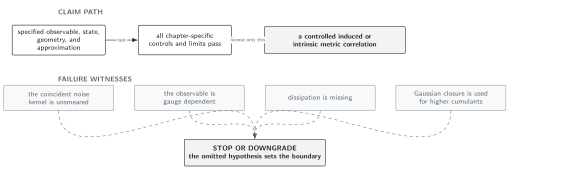
Average-time dependence is a direct diagnostic of the failed equilibrium hypothesis; a local or adiabatic approximation needs its own error estimate. The map is schematic and not to scale.

Exercises

Starting from $W^>(\omega)=e^{\beta\omega}W^<(\omega)$, derive the displayed $\coth$ factor.

Solution

Let $r=e^{\beta\omega}$. Then $N=(r+1)W^</2$ and $\rho=(r-1)W^<$. Their ratio is $(r+1)/[2(r-1)]=\frac12\coth(\beta\omega/2)$.

References

• Campos, A., and B. L. Hu. “Nonequilibrium Dynamics of a Thermal Plasma in a Gravitational Field.” Physical Review D 58, 125021 (1998). doi:10.1103/PhysRevD.58.125021. Open PDF
• Kubo, R. “Statistical-Mechanical Theory of Irreversible Processes. I.” Journal of the Physical Society of Japan 12, 570–586 (1957). doi:10.1143/JPSJ.12.570