Stationary Distributions and First-Passage Observables

A stationary density and a first-passage distribution answer different questions. The first describes probability after relaxation under a specified current condition; the second describes when a trajectory first reaches a declared boundary. Both depend on the field domain and boundary conditions, and neither by itself defines a volume-weighted measure for eternal inflation.

Required background. Langevin and Fokker–Planck dynamics fixes the stochastic calculus and probability current; stochastic coarse-graining fixes the long field and noise normalization; and Fokker–Planck evolution supplies forward and backward generators. Helpful background. Open-system noise and dissipation explains when the Markov reduction is licensed; detailed balance and fluctuation–dissipation clarifies zero-current equilibrium; and Hawking–Moss and stochastic crossover supplies the gravitational comparison.

Probability current and stationary measures

For a light spectator in fixed de Sitter space, the leading cosmic-time equation is

$$d\phi=-\frac{V'(\phi)}{3H}\,dt +\frac{H^{3/2}}{2\pi}\,dW_t, \qquad \mathbb E[dW_t^2]=dt.$$

Its density satisfies $\partial_tP=-\partial_\phi J$ with

$$J(\phi,t) =-\frac{V'}{3H}P -\frac{H^3}{8\pi^2}\partial_\phi P.$$

Setting $J=0$ gives

$$P_{\rm eq}(\phi)=\mathcal N \exp\!\left[-\frac{8\pi^2V(\phi)}{3H^4}\right].$$

This is an equilibrium result only if $H$ is constant, the density is normalizable on the declared field domain, the boundary current vanishes, and evolution lasts longer than the slowest relaxation time. A periodic field needs a periodic current condition; a noncompact field needs sufficient growth of $V$ or another specified boundary prescription. A constant nonzero current describes a nonequilibrium steady flow, not the distribution above. The result weights comoving stochastic histories. Adding physical-volume reproduction changes the evolution equation and the question, so it cannot be inferred from $P_{\rm eq}$.

The fixed-background equilibrium and spectral relaxation problem for light self-interacting scalars is derived by Starobinsky and Yokoyama 1994, §§II–IV, Eqs. (2.1)–(4.13).

First-passage boundary problem

Let $\tau$ be the first time that $\phi_t$ leaves an interval $D=(\phi_r,\phi_b)$. The survival probability is

$$S(t\mid\phi_0)=\Pr_{\phi_0}(\tau>t), \qquad f_\tau(t\mid\phi_0)=-\partial_tS,$$

and the mean hitting time $T(\phi)=\mathbb E_\phi[\tau]$ obeys the backward equation

$$\mathcal L^\dagger T =A(\phi)T'(\phi)+\frac{B^2(\phi)}2T''(\phi) =-1.$$

An absorbing endpoint imposes $T(\phi_b)=0$ because the clock stops there. A reflecting endpoint imposes $T'(\phi_r)=0$ for additive diffusion. Two absorbing endpoints instead ask which exit is reached first and require both boundary values. These are physical data, not harmless numerical choices: moving an absorbing surface changes the random variable.

First application: escape from a bounded spectator well

Take

$$V(\phi)=\frac{\lambda}{4}(\phi^2-v^2)^2, \qquad \lambda>0,$$

and study escape from the left minimum. Place a reflecting boundary sufficiently far to the left and an absorbing boundary at, or just beyond, the barrier top $\phi=0$. Solve the backward equation directly and compare it with a Langevin ensemble whose trajectories stop at the same surface. In the high-barrier, locally quadratic, overdamped Markov regime, the leading Kramers estimate is

$$\Gamma_{-v\rightarrow0} \simeq \frac{\sqrt{V''(-v)\lvert V''(0)\rvert}}{6\pi H} \exp\!\left[-\frac{8\pi^2\Delta V}{3H^4}\right], \qquad \Delta V=V(0)-V(-v).$$

The exponent is the ratio of the barrier to the effective stochastic scale $3H^4/(8\pi^2)$; the prefactor follows from the local curvatures and mobility $1/(3H)$. It is not reliable for a shallow barrier, a boundary too close to the well, colored noise, appreciable backreaction, or a transition shorter than the relaxation hierarchy. First-passage methods applied to slow-roll tunneling and multiple extrema, including their boundary-sensitive decay rates, are developed in Noorbala et al. 2018, §§3–5, Eqs. (3.1)–(5.10).

The structure map separates normalization and zero-current relaxation from absorbing-boundary observables. Inspect where the boundary data enter before interpreting a rate.

Stationarity requires normalizable zero-current evolution, whereas a hitting distribution requires declared absorbing and reflecting surfaces. Schematic; not to scale.

Domain and failure conditions

Use the chapter’s canonical domain table. The formulas above assume a single Markov coordinate, fixed $H$, additive leading noise, negligible energy transfer to the geometry, and a comoving probability density. With field-dependent $H$, multiplicative noise, curved field space, or memory, one must return to the corresponding generator and measure before imposing boundaries.

Adversarial test. Move the absorbing boundary from the barrier top to a surface on its far side and vary the reflecting cutoff until the well dynamics is insensitive to it. The exact backward solution and stopped-trajectory ensemble must agree at each placement, while the mean first-passage time should change by the calculable post-barrier travel contribution. Then shorten the available de Sitter duration. If it is not long compared with the inferred mean and relaxation times, report the finite-time survival probability rather than an asymptotic rate.

The failure map rejects equilibrium claims with nonnormalizable densities or hidden flux, and it rejects decay rates whose boundary or duration is unspecified. Time-dependent backgrounds pass to quasi-de Sitter validity; genuine gravitational saddle comparisons pass to Hawking–Moss and stochastic crossover.

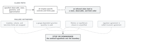
Equilibrium, hitting probabilities, and escape rates have distinct normalization, boundary, duration, and backreaction tests. Schematic; not to scale.

References

• Noorbala, M., V. Vennin, H. Assadullahi, H. Firouzjahi, and D. Wands, “Tunneling in Stochastic Inflation,” Journal of Cosmology and Astroparticle Physics 2018(09), 032 (2018), doi:10.1088/1475-7516/2018/09/032.
• Starobinsky, A. A., and J. Yokoyama, “Equilibrium State of a Self-Interacting Scalar Field in the de Sitter Background,” Physical Review D 50, 6357–6368 (1994), doi:10.1103/PhysRevD.50.6357.

References

Section titled “References”- Gillespie, D. T., “Exact Stochastic Simulation of Coupled Chemical Reactions,” The Journal of Physical Chemistry 81(25), 2340–2361 (1977), doi:10.1021/j100540a008.
- Hofmann, H., and F. A. Ivanyuk, “Mean First Passage Time for Nuclear Fission and the Emission of Light Particles,” Physical Review Letters 90, 132701 (2003), doi:10.1103/PhysRevLett.90.132701. Open PDF.