Thermal Nucleation in an Expanding Universe

A cosmological nucleation calculation takes a finite-temperature rate as versioned microscopic input and integrates it through a specified expansion and thermal history. It does not improve the rate’s perturbative accuracy, restore equilibrium after it fails, or determine the later wall motion. Its controlled output is a distribution of nucleation events with the input covariance carried intact.

Required background. False-vacuum decay with gravity distinguishes a local proper-volume rate from survival on a slice. Thermal bounce rates defines the microscopic input, and semiclassical FLRW backreaction supplies the background equations.

Helpful background. Bubble growth and wall friction supplies later wall data, while percolation, reheating, and completion supplies the downstream history problem.

The imported rate and its domain

For a locally equilibrated plasma, a common input has the form

$$\Gamma(T)=A(T)\exp\!\left[-\frac{S_3(T)}{T}\right],$$

where $\Gamma$ is a rate per physical time per physical volume. $S_3$ is the thermal critical-bubble action and $A$ includes fluctuation and dynamical information in a declared prescription. Linde derives the high-temperature $O(3)$ saddle exponent and its relation to thermal nucleation (Linde 1983, §§ 2–3).

The cosmological calculation should ingest, rather than silently reconstruct,

$$\left\{ \begin{gathered} T_i,\ \log\Gamma_i, \operatorname{Cov}(\log\Gamma_i,\log\Gamma_j),\\ p(T),\rho(T),s(T), \text{scheme and approximation tags} \end{gathered} \right\}.$$

Using $\log\Gamma$ avoids loss of precision across many decades. Joint samples must preserve correlations between neighboring temperatures and shared parameters. Varying each temperature bin independently manufactures rapidly oscillating rates that no underlying effective action could produce.

Local equilibrium requires more than $T\gg H$. Relevant plasma relaxation and bubble-formation scales must satisfy, schematically,

$$H\tau_{\mathrm{rel}}\ll1, \qquad \frac{\lvert\dot T\rvert}{T}\tau_{\mathrm{rel}}\ll1, \qquad H R_\ast\ll1,$$

where $R_\ast$ is the critical-bubble scale. If these fail, inserting an equilibrium $\Gamma(T)$ into an FLRW integral is not a controlled nonequilibrium calculation.

Radiation-dominated benchmark

In spatially flat FLRW,

$$H^2=\frac{8\pi G}{3}\rho, \qquad \dot\rho+3H(\rho+p)=0.$$

If comoving entropy is conserved and

$$s(T)=\frac{2\pi^2}{45}g_{*s}(T)T^3,$$

then

$$\frac{\dot T}{T} =-\frac{H} {1+\frac13\,d\log g_{*s}/d\log T}.$$

For constant relativistic degrees of freedom, $T\propto a^{-1}$ and $dt=-dT/(HT)$. This is the first benchmark a numerical history must reproduce.

Choose a fixed comoving region of volume $V_c$. Its instantaneous Poisson intensity is

$$\lambda(t)=V_c\,a(t)^3\Gamma[T(t)].$$

Starting at $t_i$, the no-nucleation probability and first-event density are

$$P_0(t)= \exp\!\left[-\int_{t_i}^{t}dt'\,\lambda(t')\right], \qquad p_1(t)=\lambda(t)P_0(t).$$

In the constant-$g_{*s}$ radiation benchmark, the density with respect to decreasing temperature is

$$p_1(T) =\frac{V_ca(T)^3\Gamma(T)}{H(T)T} \exp\!\left[ -\int_T^{T_i}\frac{dT'}{H(T')T'} V_ca(T')^3\Gamma(T') \right].$$

This distribution, not merely a solution of $\Gamma(T)=H(T)^4$, is the clean application. The popular equality is an order-of-magnitude onset diagnostic for one Hubble four-volume when the rate varies rapidly; it is not invariant under replacing the observation region or when $H$ and $\Gamma$ evolve slowly.

Covariance and equilibrium adversarial test

Propagate joint samples of the rate and equation of state through the time–temperature relation. For each sample, report the median and credible interval of the first-event temperature, together with the probability of no event in the chosen region. Then perform two tests:

1. retain the full supplied rate covariance and compare with an intentionally diagonalized covariance;
2. compare equilibrium evolution with a model in which $\tau_{\mathrm{rel}}\lvert\dot T\rvert/T$ approaches unity.

If the output uncertainty changes materially under covariance deletion, the diagonal treatment is rejected. If the equilibrium test fails, the answer is not a broader error bar on the same $\Gamma(T)$; it is a handoff to nonequilibrium kinetics. Caprini and collaborators summarize the distinct microscopic and cosmological inputs used in first-order-transition forecasts (Caprini et al. 2020, §§ 2.1–2.2).

Nucleation also does not imply conversion. A bubble born at $t'$ occupies a later volume determined by the wall trajectory and expansion. That spacetime overlap calculation belongs to percolation and completion.

The structure map shows the permitted direction of inference. Inspect how a versioned thermal rate and equation of state enter the expansion history before wall growth or observables are computed.

Embedding supplied thermal microphysics in an expanding universe. The diagram is schematic and not to scale; rate uncertainty and equation-of-state covariance propagate into every later transition time.

The failure map separates invalid equilibrium input from a numerical integration error. Inspect the stops associated with missing covariance, an unsupported prefactor, and a relaxation time comparable to the cooling time.

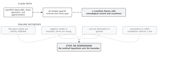
Failure conditions for cosmological rate integration. The diagram is schematic and not to scale; equilibrium breakdown requires new dynamics rather than extrapolation of the same thermal rate.

These qualifications specialize the chapter’s domain and failure conditions.

Exercise

Assume constant $g_*$ and $g_{*s}$, radiation domination, and a local rate $\Gamma(T)=\Gamma_0(T/T_0)^n$. Determine the temperature scaling of the expected number of events per Hubble four-volume, $\Gamma/H^4$.

Solution

Radiation domination gives $\rho\propto T^4$ and hence $H\propto T^2$. Therefore

$$\frac{\Gamma(T)}{H(T)^4} \propto T^{n-8}.$$

It grows as the universe cools when $n<8$, is constant when $n=8$, and decreases when $n>8$. This diagnostic does not replace the integrated first-event distribution.

References

• Caprini, C., et al. “Detecting Gravitational Waves from Cosmological Phase Transitions with LISA: An Update.” Journal of Cosmology and Astroparticle Physics 2020, no. 03 (2020): 024. DOI. Open PDF.
• Linde, A. D. “Decay of the False Vacuum at Finite Temperature.” Nuclear Physics B 216 (1983): 421–445; erratum 223 (1983): 544. DOI.