Wavefunction and Correlator Object Dictionary

A late-time wavefunction coefficient, an equal-time in-in correlator, a boundary conformal structure, and a flat-space amplitude are different objects. They can share analytic data, but only after field normalization, state, contour branches, cutoff, and continuation are fixed. This page gives the conversion that every later bootstrap statement uses.

Required background. In-in cosmological correlators and in-in contours and initial boundaries define the observable and its two branches. Celestial and cosmological handoffs distinguishes boundary data from amplitudes.

Helpful background. In-out versus in-in expectation values supplies the general distinction, and Bunch–Davies, Euclidean, and alpha states supplies the state dependence.

Wavefunction coefficients in one convention

Use

$$\int_{\mathbf k}\equiv \int\frac{d^3k}{(2\pi)^3}, \qquad \varphi_{\mathbf k}^\ast=\varphi_{-\mathbf k},$$

and define the ket wavefunctional at cutoff $\eta_0$ by

$$\begin{aligned} \Psi_{\eta_0}[\varphi] =\mathcal N\exp\Bigg[ &-\frac12\int_{\mathbf k} \Omega_k\,\varphi_{\mathbf k}\varphi_{-\mathbf k}\\ &-\sum_{n\geq3}\frac1{n!} \int_{\mathbf k_1\cdots\mathbf k_n} (2\pi)^3\delta^3\!\left(\sum_a\mathbf k_a\right) \psi_n(\{\mathbf k_a\}) \prod_a\varphi_{\mathbf k_a} \Bigg]. \end{aligned}$$

The minus signs are definitions. Authors who put $+i\psi_n$ in $\log\Psi$ use different real/imaginary and sign dictionaries. The bra branch is the complex conjugate with the conjugate analytic prescription. At tree level in a pure state, equal-time moments are

$$\langle F[\varphi]\rangle_{\eta_0} = \frac{\int\mathcal D\varphi\, \lvert\Psi_{\eta_0}[\varphi]\rvert^2F[\varphi]} {\int\mathcal D\varphi\, \lvert\Psi_{\eta_0}[\varphi]\rvert^2}.$$

For a mixed state, replace $\Psi\Psi^\ast$ by the diagonal density kernel $\rho_{\eta_0}[\varphi,\varphi]$. Off-diagonal density-matrix data still affect its evolution and cannot be reconstructed from the final diagonal alone.

Define primed correlators by removing the momentum delta function:

$$\langle\varphi_{\mathbf k_1}\cdots \varphi_{\mathbf k_n}\rangle =(2\pi)^3\delta^3\!\left(\sum_a\mathbf k_a\right) \langle\varphi_{\mathbf k_1}\cdots \varphi_{\mathbf k_n}\rangle'.$$

Gaussian inversion gives

$$P_\varphi(k) \equiv \langle\varphi_{\mathbf k}\varphi_{-\mathbf k}\rangle' =\frac1{2\operatorname{Re}\Omega_k}.$$

To first order in the cubic coefficient,

$$\langle\varphi_{\mathbf k_1} \varphi_{\mathbf k_2} \varphi_{\mathbf k_3}\rangle_c' =-2\operatorname{Re}\psi_3(\mathbf k_1,\mathbf k_2,\mathbf k_3) \prod_{a=1}^3P_\varphi(k_a).$$

The formula shows both essential facts: the observable uses both branches through a real part, and the wavefunction vertex must be amputated by the inverse Gaussian kernel. Loop corrections add contractions, normalization terms, and counterterms; the simple tree relation is not exact nonperturbatively.

Free massless scalar application

For a canonically normalized, minimally coupled massless spectator in exact de Sitter,

$$ds^2=a(\eta)^2(d\eta^2-d\mathbf x^2), \qquad a(\eta)=-\frac1{H\eta},$$

the Bunch–Davies mode is

$$u_k(\eta) =\frac{H}{\sqrt{2k^3}} (1+ik\eta)e^{-ik\eta}.$$

At $\eta_0\to0^-$,

$$\lvert u_k\rvert^2\longrightarrow\frac{H^2}{2k^3}.$$

The Schrödinger Gaussian kernel has

$$\operatorname{Re}\Omega_k \longrightarrow\frac{k^3}{H^2},$$

while its cutoff-dependent imaginary polynomial is a local phase in this example. Therefore

$$P_\varphi(k)=\frac{H^2}{2k^3}, \qquad \Delta_\varphi^2(k) \equiv\frac{k^3}{2\pi^2}P_\varphi(k) =\frac{H^2}{4\pi^2}.$$

This displays the normalization explicitly: omitting the factor of two between $\operatorname{Re}\Omega_k$ and the probability quadratic form doubles or halves the power spectrum. Maldacena uses the two-branch in-in prescription and late-time mode normalization in the inflationary calculation (Maldacena 2003, Eqs. (2.19)–(2.21) and § 3).

A massive field or alternate late-time quantization introduces two asymptotic weights and possible phases. One must say which boundary coefficient is being retained and how the late-time limit is renormalized before attaching a conformal dimension.

Boundary structures and flat-space amplitudes

A boundary conformal structure is a solution of Ward identities with assigned weights and tensor representation. It need not be the coefficient of a normalizable cosmological state, because state, branch, and positivity information are additional.

A flat-space amplitude $\mathcal A_n$ is still another object. For a local tree-level Bunch–Davies interaction, a specified total-energy singularity of $\psi_n$ can have a residue proportional to $\mathcal A_n$, with a coupling-, normalization-, power-, and phase-dependent conversion. The equality is between the appropriately normalized residue and the amplitude—not between the full $\psi_n$, the correlator, and $\mathcal A_n$. Arkani-Hamed and Maldacena exhibit this amplitude information in cosmological singularities (Arkani-Hamed and Maldacena 2015, §§ 2–3).

Phase and normalization adversarial test

Multiply the wavefunction by an allowed real local phase,

$$\Psi[\varphi]\longmapsto \exp\!\left[iS_{\mathrm{loc}}[\varphi]\right]\Psi[\varphi].$$

This shifts $\operatorname{Im}\Omega_k$ and the imaginary local parts of higher $\psi_n$, but

$$\lvert e^{iS_{\mathrm{loc}}}\Psi\rvert^2 =\lvert\Psi\rvert^2.$$

No equal-time probability effect is licensed by that shift alone. Next rescale $\chi=Z\varphi$. Then

$$\Omega_k^{(\chi)}=\frac{\Omega_k^{(\varphi)}}{Z^2}, \qquad P_\chi(k)=Z^2P_\varphi(k).$$

The coefficient and raw correlator both change, while a properly translated observable and dimensionless normalized shape agree. A claimed signal that changes under either test without an accompanying change of measured operator is conventional.

The structure map shows the inversion from one wavefunction branch to a two-branch probability observable. Inspect the distinct later route from singular residues to flat-space amplitudes.

Dictionary among wavefunction, probability, correlator, boundary, and amplitude objects. The diagram is schematic and not to scale; normalization, state, cutoff, and branch assignments are part of every conversion.

The failure map highlights convention-only effects. Inspect the stops for using one branch, dropping the factor of two, or assigning physical meaning to a removable local phase.

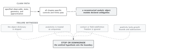
Failure conditions for cosmological object conversion. The diagram is schematic and not to scale; equal-time probabilities are invariant under allowed local phases, while coefficients remain convention dependent.

These rules specialize the chapter’s domain and failure conditions. They are the input to Ward identities and total-energy singularities.

Exercise

For one real Gaussian variable with $\Psi(x)=N\exp[-\Omega x^2/2]$ and $\operatorname{Re}\Omega>0$, compute $\langle x^2\rangle$ and check its invariance under $\Omega\mapsto\Omega+ic$ for real $c$.

Solution

The probability density is proportional to

$$\lvert\Psi(x)\rvert^2=e^{-(\operatorname{Re}\Omega)x^2}.$$

Using the Gaussian integral,

$$\langle x^2\rangle =\frac{\int dx\,x^2e^{-(\operatorname{Re}\Omega)x^2}} {\int dx\,e^{-(\operatorname{Re}\Omega)x^2}} =\frac1{2\operatorname{Re}\Omega}.$$

Adding $ic$ changes only the phase of $\Psi$ and leaves $\operatorname{Re}\Omega$, hence the variance, unchanged.

References

• Arkani-Hamed, N., and J. Maldacena. “Cosmological Collider Physics.” arXiv:1503.08043 (2015). arXiv.
• Maldacena, J. “Non-Gaussian Features of Primordial Fluctuations in Single Field Inflationary Models.” Journal of High Energy Physics 2003, no. 05 (2003): 013. DOI. Open PDF.