

Contours, iε, and Initial-Boundary Terms
An in-in contour contains physical information at its initial endpoint. Sending that endpoint to the asymptotic past with a compatible tilt projects onto an interacting vacuum under restrictive assumptions; keeping it finite requires an initial density matrix and, in an EFT, every boundary operator allowed by the remaining symmetries.
Required background. In-in cosmological correlators supplies the doubled contour; initial density matrices and boundary EFT supplies state encoding; and initial density matrices and contour boundary conditions supplies the matching equations.
Helpful background. Unitarity, normalization, and largest-time identities supplies branch-cancellation tests.
Asymptotic preparation and the iε prescription
Section titled “Asymptotic preparation and the iε prescription”For a state adiabatically connected to the free vacuum, the forward and backward branches are displaced oppositely near the remote past. Symbolically,
The tilt damps the unwanted frequency component on each branch and fixes how poles are approached. It is not interchangeable with multiplying an already divergent time integral by an arbitrary convergence factor. The interaction, the state wavefunctional, and the contour must define one analytic prescription.
For finite initial time , write
where is a boundary functional on . A Gaussian state contributes quadratic kernels within and between the two branches; non-Gaussian initial correlations produce boundary vertices. Hermiticity, normalization, and positivity constrain these kernels. Boundary conditions obtained by varying replace an informal choice of mode functions.
Concretely, Hermiticity requires , while normalization requires the full functional integral to give unity when the bulk sources coincide. Positivity is stronger than either algebraic identity: the quadratic covariance must satisfy the uncertainty relation, and non-Gaussian kernels must define a positive density operator. A set of mode functions can satisfy the Wronskian yet still fail to specify a positive mixed state if its cross-branch correlations are inconsistent.
The boundary-EFT treatment of ultraviolet state structure and its counterterms is developed in Collins and Holman 2005, §§II–V, Eqs. (2.1)–(5.18).
Boundary vertices in a cubic correlator
Section titled “Boundary vertices in a cubic correlator”As a first application, compare a cubic scalar correlator prepared in the asymptotic adiabatic vacuum with one prepared at in a Gaussian Bogoliubov state. The latter changes every bulk-to-boundary mode and can add boundary contractions. A cubic term in contributes directly at ; it is not reproduced by merely replacing the free mode function in the bulk vertex.
If a bulk integration by parts generates
the initial term combines with the state action, and the final term combines with the nonlinear definition of the measured field. Dropping both without showing their cancellation can change local momentum terms and, for a nonstandard state, physical folded-limit contributions.
The structure map displays the initial boundary as an input parallel to the bulk interaction.

State preparation is encoded either by a justified asymptotic prescription or by a finite-time boundary action whose vertices and matching conditions enter the correlator. Schematic; not to scale.
Moving the initial surface
Section titled “Moving the initial surface”Move while holding the physical state fixed. The boundary kernels must run so that a correlator at is unchanged up to the declared truncation error. This is the adversarial surface-independence test. If the result retains unsuppressed dependence on , then the boundary operator basis, its renormalization, or the assumed state preparation is incomplete.
An excited Gaussian state must also satisfy ultraviolet Hadamard or adiabatic falloff sufficient for the composite observables being computed. Otherwise bulk counterterms alone cannot renormalize the state-dependent divergences. See the chapter’s domain and failure conditions.
There is also a physical distinction between preparation and parameterization. A boundary kernel may efficiently describe an allowed state without giving a dynamical mechanism that produced it. If a claim depends on such a mechanism, its energy injection, backreaction, and correlations with fields outside the EFT must be modeled separately.
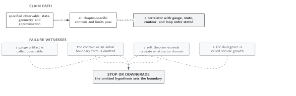
A finite-time state EFT is controlled only when its boundary conditions, vertices, ultraviolet falloff, and coefficient running remove artificial dependence on the chosen initial surface. Schematic; not to scale.
References
Section titled “References”- Collins, H., and R. Holman, “Renormalization of Initial Conditions and the Trans-Planckian Problem of Inflation,” Physical Review D 71, 085009 (2005), doi:10.1103/PhysRevD.71.085009.