Numerical Self-Consistency and Error Budgets

A numerical semiclassical solution is credible only when errors in the quantum source, geometry, coupled iteration, constraints, renormalization, and effective theory are separated. A small residual of the discretized evolution equation can coexist with a wrong continuum stress tensor or a large Hamiltonian-constraint violation. The error budget must therefore attach a convergence test and a scale to every approximation, then propagate those uncertainties to invariant observables.

Required background. Self-consistent state–geometry solutions supplies the coupled fixed point; order reduction and runaway prescriptions fixes the low-energy branch; linear response and semiclassical stability supplies conditioning diagnostics; and mode-sum numerical renormalization supplies the source calculation.

Helpful background. EFT truncation errors and breakdown diagnostics supplies theory-error estimates, while geometric discretization and continuum checks supplies tensor and mesh tests.

Residuals and errors are different quantities

Write the coupled mean equation as

$$\mathcal F[g,W]\equiv \mathcal L[g]-8\pi G\,T_{\mathrm{ren}}[g,W]=0,$$

with state equation $\mathcal P[g]W=0$ in each argument and constraints $\mathcal C[g,W]=0$. A dimensionless equation residual can be defined by

$$\mathcal R_{\mathrm{eq}} =\frac{\lVert\mathcal F[g_h,W_h]\rVert} {\lVert\mathcal L[g_h]\rVert +8\pi G\lVert T_{\mathrm{ren}}[g_h,W_h]\rVert+S_0},$$

where $S_0$ prevents an ill-conditioned zero-over-zero normalization. This measures how well the discrete pair solves the discrete equations. The solution error

$$\lVert g_h-g_{\mathrm{continuum}}\rVert$$

also depends on consistency and conditioning. Near a marginal response mode, a small source error can be amplified by a large inverse linearized operator:

$$\delta g\simeq \left(\frac{\delta\mathcal F}{\delta g}\right)_{\mathrm{ret}}^{-1} \delta T.$$

Thus residual, source error, and observable error must not be reported as synonyms.

For each run retain separate estimates for:

• spectral truncation: angular momentum, momentum, frequency, and analytic tail;
• spacetime discretization: radial mesh, time step, boundary placement, and interpolation;
• state representation: initial adiabatic order, state-mode truncation, and Wronskian/positivity residual;
• renormalization: subtraction precision, cancellation loss, analytic counterterms, and finite-coupling translation;
• nonlinear iteration: fixed-point or Newton tolerance and solver conditioning;
• constraints and conservation: Hamiltonian, momentum, $\nabla^\mu T_{\mu\nu}$, and gauge identities;
• EFT truncation: derivative order, curvature ratios, and rejected high-frequency branches; and
• roundoff and arithmetic: precision escalation in the subtracted high-frequency tail.

The structure map shows why no one entry substitutes for the others: the quantum source, causal response, constraints, branch selection, and joint state–geometry solve are successive numerical interfaces.

Propagation of numerical and theory errors through a semiclassical solve. The map is schematic and not to scale; each interface receives an independent refinement or consistency test before uncertainty is assigned to the final invariant observable.

Nested convergence for a mode-sum source

Suppose

$$T_{\mathrm{ren}}(x) =\sum_{\ell=0}^{\ell_{\max}} \left[T_\ell^{\mathrm{bare}}(x)-T_\ell^{\mathrm{sub}}(x)\right] +T_{\mathrm{tail}}(x;\ell_{\max}) +T_{\mathrm{local}}(x).$$

The bare and subtraction terms can be much larger than their difference. A convincing calculation therefore verifies the large-$\ell$ asymptotic coefficients before summation, raises arithmetic precision, and varies $\ell_{\max}$ independently of the spacetime mesh. Static black-hole stress calculations provide concrete examples of the required local subtraction, conservation, and numerical mode sum (Anderson, Hiscock, and Samuel 1995, §§ II–IV).

Use nested refinements rather than changing every parameter at once:

1. at fixed geometry and state, converge the subtracted source in $\ell_{\max}$, tail order, and precision;
2. at fixed source accuracy, refine the spacetime mesh and time integrator;
3. at each resolution, tighten the state–geometry iteration;
4. only after numerical convergence, vary adiabatic or derivative order to estimate approximation error; and
5. repeat enough of the sequence to detect cross-coupling between the dominant errors.

For an observable $Q$, a Richardson estimate for a mesh with ratio $r$ and observed order $p$ is

$$\Delta Q_{\mathrm{mesh}} \simeq\frac{\lvert Q_h-Q_{h/r}\rvert}{r^p-1}.$$

A spectral estimate may instead come from the fitted asymptotic tail. The fit window and uncertainty must be varied; agreement with a presumed power law over two points does not establish that the asymptotic regime has been reached.

Correlated contributions should not automatically be added in quadrature. A conservative first report is

$$\Delta Q_{\mathrm{tot}} \le \Delta Q_{\mathrm{spec}} +\Delta Q_{\mathrm{mesh}} +\Delta Q_{\mathrm{iter}} +\Delta Q_{\mathrm{state}} +\Delta Q_{\mathrm{ren}} +\Delta Q_{\mathrm{EFT}},$$

together with the signed shifts from each control variation. If covariance is estimated from a designed ensemble of runs, that model and sampling should be stated.

A full adversarial run

For a homogeneous backreaction calculation, monitor

$$\mathcal R_{\mathrm H} =\frac{\lvert3H^2+\Lambda+\mathcal H_{00}^{\mathrm{loc}} -8\pi G\rho_{\mathrm{ren}}\rvert}{S_{\mathrm H}}, \qquad \mathcal R_{\mathrm{cons}} =\frac{\lvert\dot\rho_{\mathrm{ren}} +3H(\rho_{\mathrm{ren}}+p_{\mathrm{ren}})\rvert}{S_{\mathrm{cons}}},$$

with nonvanishing physical scales $S_{\mathrm H}$ and $S_{\mathrm{cons}}$. Also track the mode Wronskian, the difference between successive self-consistency iterates, and the largest resolved ratio $\omega/\Lambda_{\mathrm{EFT}}$.

The adversarial case initializes the evolution with a small violation of the Hamiltonian constraint while solving the evolution equations to machine precision. A free-evolution code can retain or amplify that off-constraint component, so $\mathcal R_{\mathrm{eq}}$ remains tiny while $\mathcal R_{\mathrm H}$ is large. The run fails. Constraint projection must not conceal the issue either: report both the correction applied and the pre-projection residual.

Perform a second negative control by deliberately exciting the short-scale root removed by order reduction. Mesh convergence of that root confirms only the discrete solver. Its frequency-ratio and successive-operator tests must reject it from the EFT result.

The failure map summarizes these independent witnesses. The right-hand success node is reached only when they pass together.

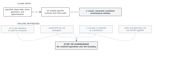
Numerical acceptance and failure paths. The map is schematic and not to scale; a small field-equation residual is one diagnostic among source convergence, Ward identities, constraints, branch control, and observable stability.

Reporting an observable

For every quoted $Q$, give the central value, units, renormalization prescription, state and geometry data, branch prescription, and a decomposed uncertainty. Also provide at least one raw convergence sequence, the norm and domain used for residuals, and the first control that limits further evolution. Invariant or orthonormal observables are preferable to coordinate components near horizons or coordinate singularities.

An uncertainty smaller than the shift under an allowed finite-coupling translation is meaningless unless the translated coupling is fixed by a renormalization condition. Similarly, an extremely precise mean geometry does not constrain the noise kernel. Numerical precision cannot promote an omitted observable into the model.

Domain and failure conditions

See the chapter domain and failure-conditions table. The workflow assumes a stable continuum formulation, a covariant subtraction, compatible state–geometry data, and a controlled EFT branch. It fails when convergence is nonuniform, cancellation exhausts arithmetic precision, boundary reflections contaminate the interval, residual norms hide localized defects, or the physical response is too ill-conditioned for the stated source uncertainty.

Exercise

A code gives $Q_h=1.040$, $Q_{h/2}=1.010$, and $Q_{h/4}=1.0025$. Estimate the observed convergence order and the remaining mesh error in $Q_{h/4}$.

Solution

The successive differences are $0.030$ and $0.0075$, whose ratio is $4=2^2$, so $p=2$. Richardson’s estimate at the finest grid is

$$\Delta Q_{\mathrm{mesh}} \simeq\frac{0.0075}{2^2-1}=0.0025.$$

This estimate addresses only mesh error; the source, iteration, constraint, and EFT entries remain separate.

References

• Anderson, P. R., W. A. Hiscock, and D. A. Samuel. “Stress-Energy Tensor of Quantized Scalar Fields in Static Spherically Symmetric Spacetimes.” Physical Review D 51 (1995): 4337–4358. DOI.
• del Río, A. “The Backreaction Problem for Black Holes in Semiclassical Gravity.” General Relativity and Gravitation 57 (2025): 30. DOI.
• Parker, L., and D. Toms. Quantum Field Theory in Curved Spacetime: Quantized Fields and Gravity. Cambridge University Press, 2009. DOI.