Parametric-Oscillator and Solvable Production Benchmarks

Exactly solvable oscillators turn particle-production approximations into falsifiable calculations. A useful benchmark fixes the normalized in-mode, exact out coefficient, number and energy observables, slow and sudden limits, and a quantitative error norm. Agreement at one parameter point does not validate WKB, Stokes, or numerics outside that domain.

Required background. Particle Creation in Time-Dependent Backgrounds supplies in/out coefficients; Adiabaticity, Stokes Phenomena, and Production Rates supplies the semiclassical approximation.

Helpful background. Special Functions from Equations and Boundary Data supplies connection formulas; Detector and instrument validation supplies comparison logic.

The tanh frequency fixture

Use

$$\omega^2(t) = \frac{\omega_{\mathrm{in}}^2+\omega_{\mathrm{out}}^2}{2} +\frac{\omega_{\mathrm{out}}^2-\omega_{\mathrm{in}}^2}{2} \tanh\frac{t}{\tau},$$

with positive asymptotic frequencies. Normalize the in-mode by

$$v_{\mathrm{in}}(t) \sim \frac{e^{-i\omega_{\mathrm{in}}t}} {\sqrt{2\omega_{\mathrm{in}}}} \quad(t\to-\infty).$$

The exact hypergeometric solution yields

$$n_{\mathrm{exact}} = \lvert\beta\rvert^2 = \frac{ \sinh^2\!\left[ \frac{\pi\tau}{2} (\omega_{\mathrm{out}}-\omega_{\mathrm{in}}) \right] }{ \sinh(\pi\tau\omega_{\mathrm{in}}) \sinh(\pi\tau\omega_{\mathrm{out}}) },$$

and $\lvert\alpha\rvert^2=1+n_{\mathrm{exact}}$. The gamma-function connection coefficients and their ultraviolet interpretation are given by Das, Galante, and Myers 2015, §2.

This fixture has three independent checks:

$$n_{\mathrm{exact}}=0 \quad\text{when}\quad \omega_{\mathrm{out}}=\omega_{\mathrm{in}},$$ $$n_{\mathrm{sudden}} = \frac{(\omega_{\mathrm{out}}-\omega_{\mathrm{in}})^2} {4\omega_{\mathrm{in}}\omega_{\mathrm{out}}} \quad\text{as}\quad \tau\to0,$$

and

$$n_{\mathrm{exact}} \sim e^{-2\pi\tau\min(\omega_{\mathrm{in}},\omega_{\mathrm{out}})}$$

up to a bounded prefactor in the large-$\tau$ regime with unequal frequencies.

First application: exact versus semiclassical production

Choose a grid spanning

$$r=\frac{\omega_{\mathrm{out}}}{\omega_{\mathrm{in}}}, \qquad \gamma=\tau\omega_{\mathrm{in}}.$$

For each point, compare $n_{\mathrm{exact}}$ with a WKB/Stokes estimate $n_{\mathrm{WKB}}$ using

$$\delta_{\log} = \left\lvert \log n_{\mathrm{WKB}} -\log n_{\mathrm{exact}} \right\rvert$$

when production is exponentially small, and

$$\delta_{\mathrm{rel}} = \frac{ \lvert n_{\mathrm{WKB}}-n_{\mathrm{exact}}\rvert }{ \max(n_{\mathrm{exact}},n_{\mathrm{floor}}) }$$

elsewhere. A floor prevents meaningless relative errors at exact zeros.

Regime	Exact control	Expected approximation behavior	Required report
No quench, $r=1$	$n=0$	Any nonzero answer is implementation error	Absolute residual and Wronskian
Slow, $\gamma\gg1$	Exponential suppression	Leading complex turning points should fix $\log n$	Exponent and prefactor errors separately
Sudden, $\gamma\ll1$ at fixed cutoff	Frequency-matching formula	Adiabatic WKB is outside domain	Compare with exact sudden coefficient
Strong contrast, $r\ll1$ or $r\gg1$	Exact formula remains finite per mode	Prefactor errors can be large	Scan both directions and energy weight

For a field, integrate the mode result twice: once for number and once with $\omega_{\mathrm{out}}$ for energy. Agreement in $n_{\mathbf k}$ over a narrow momentum range does not guarantee the integrated energy because the ultraviolet tail carries extra weight.

Cross-method checks

A numerical mode solver should preserve

$$i(v^*\dot v-\dot v^*v)=1$$

and extract $\alpha,\beta$ only after the final frequency has settled. Vary time range, step size, precision, and extraction window. Compare both the complex coefficients and $\lvert\beta\rvert^2$; phases matter for multi-pulse interference even when a single-pulse number agrees.

A detector calculation is not expected to equal $n_{\mathrm{exact}}$ at finite switching. It becomes a cross-check only after its spectral wavepacket, long-time limit, and out-mode resolution are matched to the number observable.

Adversarial extrapolation

Calibrate the leading WKB exponent at $\gamma\gg1$ and extrapolate it to $\gamma\ll1$. It misses the sudden matching result because there is no small adiabatic parameter. Alternatively, tune it on this single-transition profile and apply it to a double pulse. It misses interference unless the extra turning-point pair is included.

The strongest claim licensed by agreement on this fixture is that the implementation or approximation works over the scanned $(r,\gamma)$ domain for a single tanh transition. It does not establish accuracy for interacting fields, coalescing saddles, different ultraviolet completions, or backreacting geometries.

Construction and failure maps

The structure map is used here as a benchmark checklist: exact asymptotics, normalized modes, transition extraction, and energy translation must all agree.

The solvable fixture tests analytic, semiclassical, detector, and numerical methods over a declared parameter grid; the map is schematic and not to scale.

The failure map prevents calibration in one regime from being reported as universal validation.

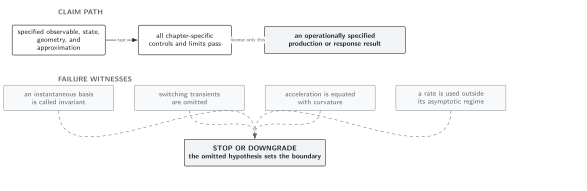
Exact agreement licenses only the scanned profile, observable, resolution, and parameter domain; out-of-domain extrapolation stops the claim. Schematic and not to scale.

Use the exact-production row in Domain and failure conditions. Report the profile, normalization, parameter grid, extraction windows, Wronskian error, coefficient identity, number and energy errors, cutoff, and every failed regime.

Check your understanding

Show the sudden limit of the exact result.

Solution

Use $\sinh x=x+O(x^3)$:

$$n_{\mathrm{exact}} \to \frac{ \left[ \pi\tau(\omega_{\mathrm{out}}-\omega_{\mathrm{in}})/2 \right]^2 }{ (\pi\tau\omega_{\mathrm{in}}) (\pi\tau\omega_{\mathrm{out}}) } = \frac{(\omega_{\mathrm{out}}-\omega_{\mathrm{in}})^2} {4\omega_{\mathrm{in}}\omega_{\mathrm{out}}}.$$

The executable calculation owns numerical sweeps and downloadable output; this page owns the analytic fixture and claim boundary. Special-function derivations remain in Volume I.

References

• N. D. Birrell and P. C. W. Davies, Quantum Fields in Curved Space, Cambridge University Press (1982), DOI, §§3.3–3.4.
• Sumit R. Das, Damián A. Galante, and Robert C. Myers, “Smooth and Fast versus Instantaneous Quenches in Quantum Field Theory,” Journal of High Energy Physics 2015 (2015), article 73, DOI, arXiv:1505.05224.
• Leonard Parker and David Toms, Quantum Field Theory in Curved Spacetime: Quantized Fields and Gravity, Cambridge University Press (2009), DOI, Chapter 2.