

Worldline Methods in Curved Space
The worldline formalism rewrites a matter heat trace as a path integral over closed particle trajectories. It is an alternative representation of the same quantum-field determinant, not a claim that the underlying field theory has been replaced by fundamental particle mechanics. In curved space the path-integral measure, the translational zero mode, spin variables, and regulator-dependent finite counterterm are essential.
Required background. One-Loop Matter Effective Actions in Curved Space fixes the determinant, and Green Operators, Causal Propagators, and State-Dependent Two-Point Functions distinguishes the Euclidean heat kernel from Lorentzian propagators.
Helpful background. Feynman and Schwinger Parameters introduces proper time, and Heat Kernels and the Schwinger–DeWitt Expansion supplies the coefficients to be reproduced.
From the heat trace to closed paths
Section titled “From the heat trace to closed paths”Use the Hamiltonian normalization
so that with . Formally,
The nonlinear sigma model contains products of distributions. In worldline dimensional regularization, with precisely this normalization, the finite counterterm is
Mode regularization and time slicing use different, partly noncovariant counterterms, but the completed transition amplitude agrees. The regulator and counterterms are tabulated in Bastianelli 2005, § 3, Eqs. (3)–(5). Quoting without the Hamiltonian normalization would be ambiguous.
Exponentiating the measure introduces commuting and anticommuting worldline ghosts. For a loop, decompose
The center is a collective coordinate; the constrained fluctuation propagator inverts the kinetic operator only on the nonzero-mode subspace. Different choices of loop center are related by a BRST treatment of this zero mode and must agree after total derivatives and measure terms are handled consistently.
First application: recover the scalar a₁ coefficient
Section titled “First application: recover the scalar a₁ coefficient”Expand the metric and curvature in Riemann normal coordinates about . Gaussian contraction of the quadratic fluctuations, measure ghosts, and the counterterm yields
for . The explicit potential contributes because it appears with the sign inherited from , while the combined kinetic, measure, ghost, and finite-counterterm graphs supply . This reproduces the heat-kernel result and vanishes at the site’s conformal coupling .
Now compute with time slicing. Its counterterm differs from by a local connection-dependent expression, and individual diagrams are not manifestly covariant. The completed coefficient must still be . If it is not, the regulator’s prescribed finite counterterm or measure ghosts have been omitted. This is the declared two-regulator adversarial check.
For spinor or -form matter, worldline Grassmann variables produce spin parallel transport and curvature couplings. Gauge systems also bring worldline gauge fixing and their own zero modes. Those constructions still evaluate matter determinants; worldline gravitons would be a different loop theory.
The structure map places the worldline path integral parallel to spectral and heat-kernel routes. Inspect the reunion at the same coefficient and determinant, rather than treating it as a new observable.

Worldline fields reorganize the matter loop; regulator counterterms and collective-coordinate fixing are required for agreement with the covariant heat kernel. Schematic; not to scale.
Domain and failure conditions
Section titled “Domain and failure conditions”The displayed formula is Euclidean, scalar, and one loop. Its target-space metric is smooth, the loop is periodic, and the center zero mode is removed. Spin, boundaries, noncompact spaces, and Lorentzian contours require additional structures. Compare methods in Domain and failure conditions.
The failure map highlights the relevant wrong turn: a bare coordinate path integral with suppressed and does not define the desired covariant Hamiltonian, even if its flat-space limit is correct.
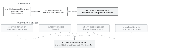
Flat-space agreement does not test the measure and ordering terms; the curved coefficient is the first decisive fixture. Schematic; not to scale.
Related topics
Section titled “Related topics”Higher local coefficients return to Seeley–DeWitt Coefficients and Curvature Invariants. Numerical coefficient generation must state the truncation, basis, recursion convention, and validation identities.