Intrinsic and Induced Metric Fluctuations

Linear stochastic metric fluctuations have two logically different origins. Intrinsic fluctuations propagate uncertainty in the initial metric data through the homogeneous semiclassical response; induced fluctuations propagate matter stress noise through the retarded Green function. Their sum is not automatic: initial matter–metric correlations generate cross terms that must either be retained or explicitly excluded by the preparation assumption.

Required background. Einstein–Langevin Dynamics fixes the stochastic equation; State–Geometry Initial Data fixes compatible initial data; and Linear Response, Stability, and Runaway Solutions supplies the stability test.

Helpful background. Initial Density Matrices and Contour Boundary Conditions explains initial correlations, while EFT Truncation Errors and Breakdown Diagnostics distinguishes physical growth from modes outside a derivative expansion.

Homogeneous and sourced solutions

Write the gauge-reduced Einstein–Langevin equation as

$$\mathcal Lh=8\pi G\,\xi.$$

For initial data $z^A$ on a Cauchy surface $\Sigma_0$, its solution is

$$h_I(x)=U_I{}^A(x)z_A +8\pi G\int_M\mathrm dV_y\, G_I^{\mathrm{ret},B}(x,y)\xi_B(y).$$

$I$ labels a physical metric component or a smeared gauge-invariant observable. The first term is intrinsic; the second is induced. Let

$$\Sigma_{AB}=\mathbb E[z_Az_B]_{\!c}, \quad N_{BC}(y,y')=\mathbb E[\xi_B(y)\xi_C(y')], \quad K_{AB}(y)=\mathbb E[z_A\xi_B(y)]_{\!c}.$$

Then the connected covariance is

$$C=C^{\mathrm{int}}+C^{\mathrm{ind}}+C^{\mathrm{cross}},$$

with

$$\begin{aligned} C^{\mathrm{int}}_{IJ}(x,x') ={}&U_I{}^A(x)\Sigma_{AB}U_J{}^B(x'),\\ C^{\mathrm{ind}}_{IJ}(x,x') ={}&(8\pi G)^2 \int\!\int G_I^{\mathrm{ret},A}(x,y) N_{AB}(y,y')G_J^{\mathrm{ret},B}(x',y'),\\ C^{\mathrm{cross}}_{IJ}(x,x') ={}&8\pi G\int U_I{}^A(x)K_{AB}(y) G_J^{\mathrm{ret},B}(x',y)+(I,x\leftrightarrow J,x'). \end{aligned}$$

Factorized initial data set $K=0$, but a common interacting preparation generally does not. Likewise, setting $\Sigma=0$ selects a sharply specified classical metric perturbation; it is not the quantum vacuum of the metric sector. The intrinsic/induced decomposition and its large-N interpretation are derived in Hu, Roura, and Verdaguer 2004, §§II–III.

The structure map should be inspected where the retarded solution splits into two inputs. Both contributions pass through the same physical response, but only the induced term contains $N$.

Intrinsic, induced, and cross covariance are separate data products; omitting one is a state-preparation choice rather than an algebraic identity. The map is schematic and not to scale.

First application: a damped gauge-invariant mode

For the stable mode

$$\ddot Q+2\gamma\dot Q+\Omega^2Q=8\pi G\,\xi, \qquad 0<\gamma<\Omega,$$

define $\omega^2=\Omega^2-\gamma^2$. The homogeneous propagation from $Q_0=Q(0)$ and $P_0=\dot Q(0)$ is

$$Q_{\mathrm{hom}}(t)=u(t)Q_0+v(t)P_0,$$

where

$$u(t)=e^{-\gamma t} \left(\cos\omega t+\frac{\gamma}{\omega}\sin\omega t\right), \qquad v(t)=e^{-\gamma t}\frac{\sin\omega t}{\omega}.$$

For initial covariance entries $\sigma_{QQ}$, $\sigma_{QP}$, and $\sigma_{PP}$,

$$C^{\mathrm{int}}(t,t') =u(t)u(t')\sigma_{QQ} +[u(t)v(t')+v(t)u(t')]\sigma_{QP} +v(t)v(t')\sigma_{PP}.$$

Every term decays as $e^{-\gamma(t+t')}$. If the projected source is approximately white over the response band,

$$\mathbb E[\xi(t)\xi(t')]=\mathcal N\delta(t-t'),$$

then, with $K=0$, the induced equal-time covariance approaches

$$C^{\mathrm{ind}}(t,t) \longrightarrow \frac{(8\pi G)^2\mathcal N}{4\gamma\Omega^2}.$$

Thus late-time loss of memory of the initial covariance does not mean the mode becomes noiseless: the intrinsic part decays while the driven part reaches a stationary value. For colored quantum noise the same conclusion is tested with $(8\pi G)^2\int\mathrm d\omega\,|G^{\mathrm{ret}}(\omega)|^2N(\omega)/(2\pi)$ rather than the white approximation.

The unstable-mode test

Replace $\Omega^2$ by $-\lambda^2$ with $\lambda>0$. One homogeneous exponent is

$$r_+=-\gamma+\sqrt{\gamma^2+\lambda^2}>0.$$

Any nonzero projection of $\Sigma$ on that mode grows as $e^{r_+(t+t')}$. Making $\mathcal N$ small does not remove this intrinsic instability; the noise-driven term also samples the growing retarded Green function. The correct conclusion is that the background or the chosen treatment of higher derivatives fails its stability domain, not that stochastic forcing dynamically repairs it.

Secular growth can be physical, a gauge artifact, an initial-state transient, or a sign of nonuniform perturbation theory. One must compare it with the curvature radius, EFT cutoff, observation duration, and neglected nonlinear terms before extrapolating.

Domain and failure conditions

The chapter comparison table licenses a covariance only after the initial metric state, matter state, cross correlations, constraint surface, retarded prescription, and stability interval are stated. A decomposition computed in one gauge must be projected to physical observables before comparison. It does not reconstruct a full quantum-gravity state from second moments.

The failure map’s instability and full-state branches are independent: bounded covariance is necessary for the linear approximation, while bounded second moments still do not determine commutators or higher quantum correlations.

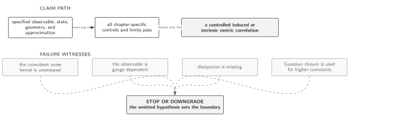
Small induced noise cannot rescue an intrinsically unstable background; stability and information completeness are separate conditions. The map is schematic and not to scale.

Exercises

Why does $K=0$ follow for a factorized initial probability functional but not for an interacting equilibrium preparation?

Solution

If the initial metric variables and matter variables are statistically independent, every connected mixed moment factorizes to zero, so $K_{AB}=\mathbb E[z_A\xi_B]-\mathbb E[z_A]\mathbb E[\xi_B]=0$. An interacting equilibrium state is a state of the coupled system and generally contains correlations across that split; tracing it into separate marginals loses precisely the data encoded by $K$.

References

• Hu, B. L., A. Roura, and E. Verdaguer. “Induced Quantum Metric Fluctuations and the Validity of Semiclassical Gravity.” Physical Review D 70, 044002 (2004). doi:10.1103/PhysRevD.70.044002. Open PDF