Fixed-Background, Semiclassical, Gravitational-EFT, and Quantum-Gravity Regimes

The boundary between fixed-background QFT, semiclassical gravity, gravitational effective field theory, and quantum gravity is determined by what is dynamical and quantized, which observable is requested, and which expansion controls the omitted terms. Curvature alone does not decide the regime. A low-curvature experiment can probe quantum metric fluctuations at sufficiently high energy or sensitivity, while a quantum field on a highly curved but prescribed background can still be a mathematically definite fixed-background model.

This page supplies a classification that should be applied before any curved-spacetime calculation. Detailed graviton-loop calculations belong to the gravitational-EFT chapter, and detailed quantum-gravity models belong to Volume XV.

Required background. Effective Field Theory as a Controlled Expansion supplies the relation among retained operators, small parameters, and truncation error used below.

Helpful background. EFT Truncation Errors and Breakdown Diagnostics develops quantitative remainder estimates; Claim–Evidence Records, Replication, and Retraction Handling helps distinguish a theoretical validity statement from empirical support.

What is prescribed and what is quantized

Write the metric as $g_{\mu\nu}$, the matter fields collectively as $\Phi$, and the requested observable as $\mathcal O$. The four useful low-energy layers are:

Layer	Metric	Matter	Typical output	Expansion that must be controlled
Fixed-background QFT	Prescribed classical field	Quantized	Correlators, detector response, $\langle T_{\mu\nu}\rangle$ on the chosen $g$	Matter coupling, loops, derivatives, state and duration
Semiclassical mean gravity	Classical field solved self-consistently	Quantized through expectation values	Mean geometry and mean matter observables	$G\langle T\rangle$, matter loops, derivatives, higher-curvature terms
Stochastic or large-$N$ gravity	Classical mean plus controlled fluctuations	Quantized stress cumulants	Symmetrized metric correlations in a stated approximation	$1/N$, fluctuation order, smearing, linear response
Gravitational EFT	Metric perturbations may be quantized	Matter and metric modes below a cutoff	Gauge-invariant low-energy amplitudes or relational observables	$E/\Lambda$, curvature/threshold scales, graviton and matter loops

“Quantum gravity” is required when the observable cannot be predicted to its target accuracy by any controlled version of these layers. That statement is observable-specific. It does not follow merely from a coordinate component becoming large or from an invariant reaching an unnamed “Planckian” value.

Several dimensionless quantities can matter simultaneously. For a characteristic curvature scale $\mathcal R$, probe energy $E$, EFT cutoff $\Lambda$, duration $\Delta t$, matter coupling $g$, and $N$ comparable species, representative parameters are

$$\epsilon_R=\frac{\mathcal R}{\Lambda^2}, \qquad \epsilon_E=\frac{E}{\Lambda}, \qquad \epsilon_G=G E^2, \qquad \epsilon_t=\Gamma\Delta t, \qquad \epsilon_N=\frac1N.$$

The loop parameter and derivative expansion depend on the theory and observable and must be stated locally. The fact that each displayed parameter is small is not by itself sufficient when a secular factor, large occupation number, or infrared enhancement compensates it.

A scalar source through five descriptions

Consider a real scalar with action

$$S_\phi[g,\phi] = \frac12\int \mathrm d^4x\sqrt{-g} \left[ g^{\mu\nu}\nabla_\mu\phi\nabla_\nu\phi -(m^2+\xi R)\phi^2 \right].$$

On a prescribed weakly curved metric, quantize $\phi$ and compute a two-point function or a renormalized stress expectation value. Integrating out $\phi$ produces a matter determinant $\Gamma_{\rm m}[g]$; it is still a fixed-background matter-loop calculation until the metric equation is varied and solved. This distinction is emphasized in the effective-action treatment of curved-space QFT Hollands and Wald 2015, §§3–4.

At semiclassical mean level, the schematic equation is

$$G_{\mu\nu}+\Lambda g_{\mu\nu} +\sum_i c_i H^{(i)}_{\mu\nu} =8\pi G\,\langle T_{\mu\nu}\rangle_{\rm ren},$$

with the state, finite gravitational couplings, initial data, and causal prescription supplied. The tensors $H^{(i)}_{\mu\nu}$ arise from local higher-curvature terms. This equation predicts a mean metric; it does not predict the full quantum distribution of metric observables.

At the next controlled layer, the connected stress covariance

$$N_{\mu\nu\rho\sigma}(x,y) = \frac12 \left\langle \left\{ t_{\mu\nu}(x),t_{\rho\sigma}(y) \right\} \right\rangle, \qquad t_{\mu\nu}=T_{\mu\nu}-\langle T_{\mu\nu}\rangle,$$

can source an Einstein–Langevin description after smearing, renormalization, and gauge-invariant projection. Stochastic gravity reproduces a specified sector of symmetrized correlations in controlled large-$N$ or linearized settings; it is not synonymous with quantizing the metric Hu and Verdaguer 2020, §§3–5.

Finally, quantizing metric perturbations introduces graviton and ghost loops. Their power counting and observables belong to Gravity as Effective Field Theory. A matter loop containing curvature tensors does not become a graviton loop merely because its answer depends on $g_{\mu\nu}$.

Why curvature cannot be the only cutoff

Hold a weak background curvature $\mathcal R$ fixed. Now vary four independent features:

• Increasing $E$ can make $GE^2$ or $E/\Lambda$ large without changing $\mathcal R$.
• Increasing $N$ enhances matter vacuum polarization while suppressing some relative fluctuations, depending on how $NG$ is scaled.
• Changing loop order distinguishes a classical background calculation from a graviton-loop observable at the same curvature.
• Changing the smearing scale can make a stress-fluctuation observable controlled or ill-defined while leaving its mean unchanged.

Therefore no threshold of the form “$\mathcal R$ reaches the Planck scale” can classify every requested observable. The correct output is a remainder estimate or a precise failure statement, not a universal label. Donoghue’s low-energy treatment makes the same point constructively: quantum gravity has model-independent low-energy predictions when the nonanalytic terms and EFT expansion are controlled, even though the ultraviolet completion is unknown Donoghue 1994, §§2–4.

A usable decision procedure

1. Name $\mathcal O$ and its resolution, duration, and required accuracy.
2. List the dynamical variables and which of them are quantized.
3. State the state or density matrix and the causal prescription.
4. List curvature, derivative, coupling, loop, $G$, $\hbar$, $1/N$, and secular parameters that can affect $\mathcal O$.
5. Bound the first omitted term or identify why it cannot be bounded.
6. Test gauge, scheme, state, and smearing dependence at the claimed order.
7. Move to a deeper regime only when the target error cannot be met within the current one.

This procedure can classify two observables on the same background differently. A mean detector response may remain a fixed-background calculation while a metric two-point function already requires a stochastic or graviton-EFT treatment.

Construction and failure maps

In the construction map, the regime is the first input, not a label added after a calculation. Inspect how that choice determines which background and field variables enter the later operator, algebra, and state-dependent steps.

Fixed-background, semiclassical, stochastic, and gravitational-EFT calculations enter the common construction with different dynamical variables and error controls; the map is schematic and not to scale.

For this page, the failure map asks whether every small parameter relevant to the named observable has been tested. Fixed curvature does not fix probe energy, loop order, duration, species number, or smearing scale.

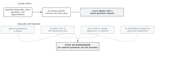
A regime classification licenses only the observable and target accuracy for which the stated expansion and remainder checks pass; the map is schematic and not to scale.

The cross-field comparison appears in Domain and failure conditions. The page-specific assumptions are the quantized variables, observable, state, scales, and truncation order; an uncontrolled first omitted term forces a narrower accuracy claim or a deeper description.

Exercise

A calculation evaluates a scalar determinant on a prescribed Schwarzschild metric and retains terms through order $R^2/m^2$. Has it computed one-loop quantum gravity?

Solution

No. It has computed a one-loop matter effective action on a prescribed metric. The curvature expansion is controlled only when derivatives and curvature are small compared with the matter threshold. It becomes a semiclassical mean calculation if the resulting action is varied in a causal framework and the metric is solved self-consistently. It contains graviton loops only if metric fluctuations and their gauge/ghost sector are integrated over.

References

• John F. Donoghue, “General Relativity as an Effective Field Theory: The Leading Quantum Corrections,” Physical Review D 50 (1994), 3874–3888, DOI, Open PDF.
• Bei-Lok Hu and Enric Verdaguer, “Stochastic Gravity: Theory and Applications,” Living Reviews in Relativity 23 (2020), article 3, DOI, arXiv:2005.13047.
• Stefan Hollands and Robert M. Wald, “Quantum Fields in Curved Spacetime,” Physics Reports 574 (2015), 1–35, DOI, Open PDF.