Real-Time Vacuum Decay and State Dependence

Real-time vacuum decay is an initial-value problem. A density matrix, a false-sector observable, a Cauchy surface, and a clock define a survival probability; the local potential alone does not. Euclidean saddles can approximate an exponential regime of that probability under additional analytic and state-preparation hypotheses, but they are not a substitute for defining it.

Required background. False-vacuum decay with gravity fixes the observable and geometric regime. Causal in-in backreaction, in-out versus in-in quantities, and closed-time-path generating functionals supply the real-time formalism.

Helpful background. Coleman–De Luccia bounces and gravitational decay prefactors identify the Euclidean quantities that may be compared.

Survival as a specified observable

Let $\Sigma_0$ be the preparation surface, $\rho_F$ a normalized state supported in a declared false sector, and $\Pi_F(t)$ the projector or positive operator that tests that sector on a later slice. Then

$$P_F(t) =\operatorname{Tr}\!\left[ \Pi_F(t)\,U(t,0)\rho_FU^\dagger(t,0) \right], \qquad 0\leq P_F\leq1 .$$

The instantaneous hazard, where $P_F>0$, is

$$\gamma(t)=-\frac{d}{dt}\log P_F(t).$$

A constant “decay rate” exists only on an interval where $\gamma(t)$ has a controlled plateau. It is generally not constant at very short times. For a pure state and survival in its initial ray,

$$P_F(t)=1-(\Delta H)^2t^2+O(t^4),$$

so $\dot P_F(0)=0$, provided the state has a finite fourth energy moment for the displayed remainder. Finite-volume recurrences and late-time spectral tails also obstruct an exact exponential for all time. None of these facts denies a long, useful exponential window; they specify what has to be demonstrated.

In quantum field theory, a sharp global projector may be impractical. Alternatives include a coarse-grained field range in a finite region, the probability distribution of a smeared order parameter, or a first-passage functional. The region, smearing, and time slicing then belong to the observable. By contrast, a local decay density $\Gamma(x)$ is defined so that, in a dilute Poisson regime,

$$P_F(\mathcal R) \simeq \exp\!\left[-\int_{\mathcal R}d^4x\,\sqrt{-g}\, \Gamma(x)\right].$$

This proper-four-volume formula is covariant; the survival probability of an extended slice is state- and foliation-dependent.

Closed-time-path evolution

For a source coupled as $S_L\mapsto S_L+\int J\mathcal O$, the normalized closed-time-path functional is

$$Z[J_+,J_-] =\operatorname{Tr}\!\left[ U_{J_+}(t_f,0)\rho_F U_{J_-}^\dagger(t_f,0) \right], \qquad Z[J,J]=1.$$

Functional derivatives with respect to $J_+$ and $J_-$ generate real-time ordered, anti-ordered, and mixed correlators. With the stated plus-action source convention, linear response is

$$\frac{\delta\langle A(t)\rangle}{\delta J(t')} =i\,\theta(t-t')\langle[A(t),\mathcal O(t')]\rangle .$$

The equality $Z[J,J]=1$ encodes unitarity and is a powerful numerical check. The in-in effective equations obtained by setting the two branches equal after variation are causal. An in-out effective action instead computes an amplitude between boundary states and can be complex even when it is not a survival probability. Jordan gives the closed-time-path construction of causal expectation-value equations (Jordan 1986, Eqs. (2.1)–(2.19)).

For a minisuperspace coordinate $q$ with false region $F=(-\infty,q_b)$, a prepared wavefunction gives

$$P_F(t)=\int_{-\infty}^{q_b}dq\,\lvert\psi(q,t)\rvert^2, \qquad -\dot P_F(t)=j(q_b,t),$$

provided the current is oriented out of $F$. This benchmark exposes normalization, early-time transients, reflections, and recrossings directly. A Euclidean exponent $B$ is comparable to the plateau hazard only if the state is quasistationary, the barrier is semiclassical, reflections are negligible, and the same false boundary is used.

State-dependence adversarial test

Prepare two Hadamard states with the same mean field and the same local effective potential near the false minimum, but different ultraviolet-safe occupation profiles. Evolve both with the same Hamiltonian and false-sector test. Their connected correlators, energy density, barrier-crossing flux, and $\gamma(t)$ need not agree.

A robust claim reports:

$$\rho_F,\quad \Pi_F,\quad \Sigma_0,\quad \text{clock},\quad \text{coarse graining},\quad [t_1,t_2]_{\mathrm{plateau}},$$

together with regulator and volume convergence. If the two preparations produce different plateau rates, the difference is physical state dependence. If the difference disappears only after changing the false-sector boundary, the observable was not held fixed.

Batini, Chatrchyan, and Berges find explicitly time-dependent false-vacuum decay rates at next-to-leading order in a large-$N$ two-particle-irreducible treatment, providing a controlled field-theory example of this initial-value structure (Batini, Chatrchyan, and Berges 2024, §§ II, V–VI). That controlled model is evidence about real-time dynamics, not a proof that the same approximation controls gravitational decay.

The structure map shows that state preparation and causal evolution are parallel to, rather than hidden inside, the Euclidean route. Inspect the point where a plateau hazard may be compared with a saddle exponent.

Real-time state preparation, unitary evolution, and the restricted comparison with a Euclidean saddle. The diagram is schematic and not to scale; the prepared state and false-sector observable remain explicit inputs.

The failure map identifies non-exponential evolution and unmatched states as stopping conditions. A fit to one short interval is not a universal rate if it changes with the preparation, volume, or coarse-graining boundary.

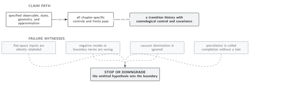
Failure conditions for a Lorentzian survival calculation. The diagram is schematic and not to scale; potential data alone cannot determine a state-dependent hazard.

These limits refine the chapter’s domain and failure conditions. A supplied thermal rate enters cosmology only at thermal nucleation in an expanding universe.

Exercise

Suppose $P_F(t)=Ze^{-\gamma t}+ce^{-2\gamma t}$ with $Z>0$ and $\lvert c\rvert e^{-\gamma t}\ll Z$. Find the leading departure of the instantaneous hazard from $\gamma$.

Solution

Factor $P_F=Ze^{-\gamma t}[1+(c/Z)e^{-\gamma t}]$. Therefore

$$-\frac{d}{dt}\log P_F =\gamma+ \gamma\frac{(c/Z)e^{-\gamma t}} {1+(c/Z)e^{-\gamma t}} =\gamma+\gamma\frac{c}{Z}e^{-\gamma t} +O(e^{-2\gamma t}).$$

The fitted rate approaches $\gamma$ only after the transient term is small; the sign of the approach depends on $c$.

References

• Batini, L., A. Chatrchyan, and J. Berges. “Real-Time Dynamics of False Vacuum Decay.” Physical Review D 109 (2024): 023502. DOI. Open PDF.
• Jordan, R. D. “Effective Field Equations for Expectation Values.” Physical Review D 33 (1986): 444–454. DOI.