

Curved Spacetimes, Cauchy Surfaces, and Global Hyperbolicity
A local hyperbolic field equation becomes a globally predictive initial-value problem when the spacetime has an appropriate causal structure and the initial hypersurface is Cauchy. Global hyperbolicity is the standard boundary-free hypothesis: it excludes closed causal curves, controls causal diamonds, and ensures that every inextendible causal curve meets a Cauchy surface exactly once. If a timelike boundary or chronology-violating region is present, the differential equation may remain locally hyperbolic while global evolution requires extra data or fails altogether.
Required background. Smooth Manifolds, Tangent and Cotangent Bundles, and Tensor Fields supplies hypersurfaces and tensor fields; Bundle Connections, Curvature, Gauge Transformations, and Bianchi Identities supplies covariant differentiation.
Helpful background. Levi–Civita Connections, Geodesics, and Riemann Curvature supplies geodesic geometry; Hyperbolic Equations and Causal Propagators supplies the analytic consequences used below.
Causal structure and Cauchy data
Section titled “Causal structure and Cauchy data”Let be a connected, time-oriented Lorentzian manifold without boundary. For , and denote the points reachable from by future- and past-directed causal curves. The causal diamond between and is
A subset is a Cauchy surface if every inextendible timelike curve meets exactly once. Under the usual causality hypotheses this is equivalent to the corresponding statement for inextendible causal curves. Initial data on then intersect every possible causal history once, which is the geometric reason they can determine a global solution.
A spacetime is globally hyperbolic when it is causal and every diamond is compact. Equivalent formulations use strong causality or non-total imprisonment together with compact diamonds. A fundamental structure theorem says that a globally hyperbolic spacetime admits a smooth Cauchy temporal function and a splitting
where each slice is a smooth spacelike Cauchy surface and is Riemannian. Bernal and Sánchez prove the smooth splitting and smoothability results with the relevant causal hypotheses Bernal and Sánchez 2005, Theorems 1.1–1.2.
Global hyperbolicity is global: no curvature scalar at one point detects it. Minkowski spacetime and a flat spacetime with periodic time have identical local curvature, but the latter contains closed timelike curves and has no Cauchy surface.
What the hypothesis buys for a field equation
Section titled “What the hypothesis buys for a field equation”Let be a normally hyperbolic operator on a vector bundle, with principal symbol
On a globally hyperbolic spacetime, smooth compactly supported source and compactly supported Cauchy data determine a unique smooth solution of
where is the future unit normal. The solution depends continuously on the data and has finite propagation speed: its support lies in the causal development of the source and initial support. Bär, Ginoux, and Pfäffle state the well-posedness and support result precisely in Theorems 3.2.11–3.2.12 Open PDF.
The same hypotheses yield unique retarded and advanced Green operators on compactly supported sources. These are analytic consequences of the geometry plus the operator class; they are not definitions of a vacuum or of particle number.
For the Klein–Gordon field, and . For a first-order Dirac equation only the appropriate spinor datum is specified. Gauge systems add constraint equations and quotient data. Thus “Cauchy surface” does not mean that every field accepts the same freely specifiable pair of functions.
Three scalar initial-value problems
Section titled “Three scalar initial-value problems”Consider .
| Background | Candidate initial surface | Data needed for prediction | Conclusion |
|---|---|---|---|
| Minkowski spacetime | with suitable regularity | Globally hyperbolic; unique global solution | |
| Spatially flat FLRW, , with on its time interval | Each slice is Cauchy for the stated spacetime; singular endpoints are not included | ||
| A region with timelike boundary | Spacelike slice ending on the boundary | Initial data and a boundary condition with compatible corner data | Ordinary boundary-free global-hyperbolicity theorem does not establish uniqueness |
The FLRW statement does not claim that evolution extends through a big-bang singularity. It says that the manifold on its declared open time interval has Cauchy slices. Predicting beyond an endpoint requires a new spacetime extension and new physical input.
The timelike-boundary case illustrates why local characteristics are insufficient. A signal can leave the initial domain, reach the boundary, and return. Dirichlet, Neumann, Robin, transparent, or dynamical boundary conditions describe different systems and generally give different Green operators.
Removing the decisive hypothesis
Section titled “Removing the decisive hypothesis”Start with two-dimensional Minkowski spacetime and identify . Every point then lies on a closed timelike curve. The Klein–Gordon operator retains the same local principal symbol, but no hypersurface can meet each inextendible timelike curve exactly once. Prescribing data on a local spacelike segment therefore does not define an unrestricted global evolution.
A milder failure occurs in anti-de Sitter spacetime: there need not be closed timelike curves on the universal cover, but causal curves can reach conformal infinity and return in finite time. Additional boundary conditions can define predictive dynamics, yet the result is a chosen initial-boundary theory rather than an application of the boundary-free theorem. The self-adjoint-extension analysis is developed on the dedicated boundary page.
Stop rule. Do not infer a unique global propagator from the local phrase “normally hyperbolic.” Verify the spacetime domain, Cauchy or boundary data, operator realization, and support class first.
Construction and failure maps
Section titled “Construction and failure maps”The first diagram begins with the causal domain because every later Green operator, conserved solution space, and local algebra depends on it. On this page, the decisive input is a Cauchy surface for the entire domain under discussion.

Global hyperbolicity supplies the predictive causal stage of the chapter’s construction; the map is schematic and not to scale.
In the second diagram, inspect the first failure witness. Closed timelike curves, a naked timelike boundary, or noncompact causal diamonds can invalidate the standard Cauchy theorem even when the differential equation is locally hyperbolic.
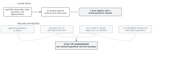
Local hyperbolicity alone does not license global evolution; a missing Cauchy hypothesis requires a boundary-sensitive replacement or a restricted domain. Schematic and not to scale.
The field-by-field comparison is in Domain and failure conditions. Here one must verify causality, compact diamonds or an equivalent criterion, completeness of the Cauchy data, and absence of uncontrolled boundary flux.
Exercise
Section titled “Exercise”Why is a constant- hyperplane in Minkowski spacetime Cauchy, while a constant- segment in a finite spatial strip is not sufficient by itself?
Solution
Every inextendible causal curve in Minkowski spacetime has time coordinate ranging from to and therefore crosses the hyperplane once. In a finite strip, causal curves can encounter a timelike side boundary. Initial data on the segment do not say what enters from, reflects from, or is absorbed by that boundary, so a boundary condition and compatible corner data are also required.
References
Section titled “References”- Christian Bär, Nicolas Ginoux, and Frank Pfäffle, Wave Equations on Lorentzian Manifolds and Quantization, European Mathematical Society (2007), Open PDF, §§3.2–3.4.
- Antonio N. Bernal and Miguel Sánchez, “Smoothness of Time Functions and the Metric Splitting of Globally Hyperbolic Spacetimes,” Communications in Mathematical Physics 257 (2005), 43–50, DOI, arXiv:gr-qc/0401112.
- Robert M. Wald, Quantum Field Theory in Curved Spacetime and Black Hole Thermodynamics, University of Chicago Press (1994), Chapter 3, publisher record.